Marathon Data Via RSelenium

A while back I showed how to use a cell phone as an activity tracker. Part of the reason behind this was that I thought it would make me run more. If you look on my projects page I mentioned how this was going to help me train for a 5k.

I am not sure how much I actually used this to train, very little I would guess, but I did end up running the DC Race4Respect 5k. After the race I wanted to look at the results, and more than just the table they give you on the webpage. Getting the data for this race was a little strange though as can be seen here. It could not be collected with the normal use of httr, XML and rvest. It required the RSelenium package to automate the clicks, this is due to the data being hid behind javascript. I have used this a few times, but every time it seems I need to re-read what I have done before or Google around a bit to find the correct setup.

Here I want to document some of the setup and process for using RSelenium, it may save me some time on the next go around. I have had issues with this before where everything I could find on RSelenium failed because it was written for Windows. To get around this on Mac I have to use phantomjs, a headless browser as none of the browsers I have installed seem to work.

options(stringsAsFactors = FALSE)
library(RSelenium)
library(ggplot2)
require(beanplot)
library(dplyr)
library(lubridate)
library(XML)

info <- list()

get_cur_data <- function() {
  readHTMLTable(remDr$findElement(using = 'id', 
                                  value = "bazu-full-results-grid"
  )$getElementAttribute("outerHTML")[[1]])[[1]]
}

goto_page <- function(val) {
  remDr$findElements(using = 'class name', 
                   value = "fg-button")[[val]]$sendKeysToElement(list(key = "enter"))
}

# Setup the selenium and phantom.js
startServer()
phanDir <- "/Users/kdarrell/node_modules/phantomjs/lib/phantom/bin/phantomjs"
  
# Create phantomjs driver, needs location of exe
remDr <- remoteDriver(browserName = "phantomjs", 
                      extraCapabilities = list(phantomjs.binary.path = phanDir))

Once this is all setup with the headless browser it does not deviate very much from the tutorials. You can see how imperative the code is. With a few helper functions it actually reads as though you are describing how you clicked around on the page.

# Open a connection to the remote driver, open browser
remDr$open()
  
race_url <- 'http://results.chronotrack.com/event/results/event/event-14387'
# Start at the race results page.
remDr$navigate(race_url)
 
#remDr$screenshot(display = TRUE, useViewer = TRUE) 

# Locate the element that links to results.
webElem <- remDr$findElement(using = 'id', value = "resultsResultsTab")

# Click button on this 
webElem$sendKeysToElement(list(key = "enter"))
  
# Collect info on first page
info[[length(info) + 1]] <- get_cur_data()

goto_page(4)    # Go to page 2
info[[length(info) + 1]] <- get_cur_data()

goto_page(5)    # Go to page 3
info[[length(info) + 1]] <- get_cur_data()

goto_page(6)    # Go to page 4
info[[length(info) + 1]] <- get_cur_data()

# Loop through the rest
for (i in 5:46) {
  goto_page(6)
  info[[length(info) + 1]] <- get_cur_data()
}

goto_page(7)   # Go to the last page
info[[length(info) + 1]] <- get_cur_data()

# Turn list into data.frame
r4r5k <- as.data.frame(bind_rows(info))

A few things to note, it may appear that there is a bug and that I should use goto_page at the increment variable. This is however the item that will jump to the next page, not actually the page I am jumping to.

This would all be rather dull without some use of this data. The following code will take a subset of the fields from a race and create a beanplot. This is a collection of back to back histograms, using a binary indicatory, over another categorical variable. In this case we can see the distribution of minutes it took to finish the race for sex and age.

raceplot <- function(data, t = 'Race') {
  beanplot(data$min ~ data$sex * data$group, ll = 0.04, side = "both",   
           col = list("purple", c("lightblue", "black")),         
           main = paste0(t, " Minutes by Age/Sex"), 
           axes = F, log = '')
  
  axis(1, at = c(1:8), labels = c("10s", "20s", "30s", "40s", 
                                  "50s", "60s", "70s", "80s"))
  
  axis(2)
  legend("bottomleft", fill = c("purple", "lightblue"),       
         legend = c("Female", "Male"), box.lty = 0)
}

# Turn tace times into minutes as numeric.
time_2_min <- function(x) {
  x <- strsplit(x, ':')
  sec <- as.numeric(sapply(x, `[`, 1)) * 60 * 60 +
    as.numeric(sapply(x, `[`, 2)) * 60 + as.numeric(sapply(x, `[`, 3))
  sec / 60
}

Now the only step is to contort the data into the desired format.

r4r5k %>%
  mutate(min = time_2_min(Time),
         age = as.numeric(Age)) %>%
  select(age, min, sex = Gender) %>%
  filter(age > 9, age < 90) %>%
  mutate(group = as.factor(floor(age/10))) %>%
  raceplot('5K')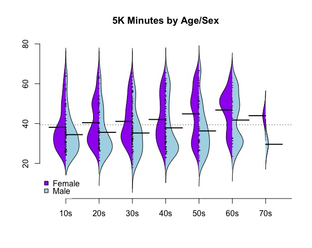

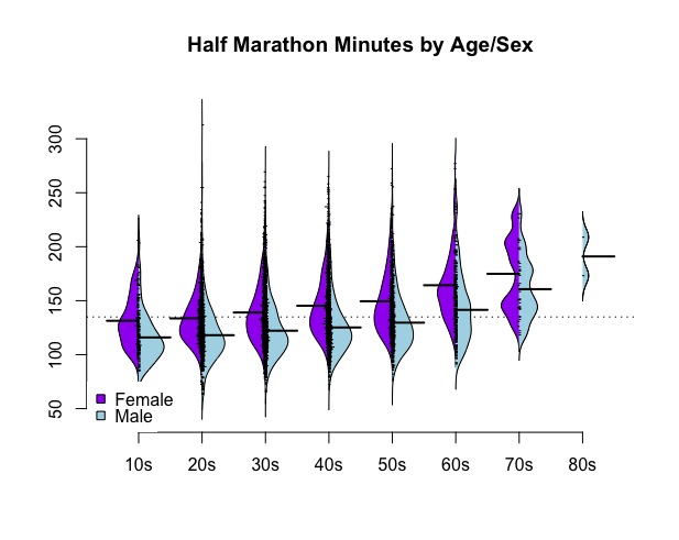
I also ran the Anthem Richmon Half-Marathon. The data was sitting behind the same type of javascript code, so collecting it required the same mechanism. This was much easier to put in a loop so it does not read as a sequence of clicks. This is because it had number indicating what page to start on. It was also much much harder because I could never get it to work on a Mac. I tried it on a Windows machine and everything worked, no need for phantomjs.

# This only worked on Windows.
base <- 'http://www.richmond.com/data-center/marathon/2015/'
ext <- '?PageID=2&PrevPageID=&cpipage='

startServer()
data <- list()
mybrowser <- remoteDriver()

mybrowser$open()

for (i in 1:315) {
  Sys.sleep(runif(1, 7, 12))
  mybrowser$navigate(paste0(base, ext, i))
  x <- mybrowser$findElements(using = 'tag', "tr")
  
  data[[i]] <- sapply(x, function(i) i$getElementText()[[1]])
  tail(data[[i]], 1)
}
save(data, file = 'anthem.RData')

Same thing for this data, contort it into the desired format and then plot.

data %>% unlist %>%
  grep('Records ', ., value = T, invert = T)  %>% 
  grep('Last Name ', ., value = T, invert = T)  %>%
  grep('Page     of 315 ', ., value = T, invert = T) %>%
  { .[. != ''] } %>%
  strsplit(., ' ') %>%
  sapply(tail, 5) %>% t %>%
  as.data.frame(stringsAsFactors = FALSE)  %>%
  select(sex = V1, age = V2, race = V3, min = V5) %>%
  mutate(min = time_2_min(min),
         age = as.numeric(age)) %>%
  filter(age > 9, age < 90, race == 'HM') %>%
  mutate(group = as.factor(floor(age/10))) %>%
  raceplot('Half Marathon')