Making Your Own Activity Tracker

Background

This post is the culmination of a few ideas. When I was an undergraduate and the the early part of my career where I was an Aerospace Engineer and a Control Systems Engineer I worked with lots of sensors. These sensors streamed in lots of data in the form of measurements of certain features of the real world. This part of the job was really cool. There were other really cool parts as well, I was doing a lot of data mining and machine learning before I even knew what those thing were. There are other parts of being an engineer that I did not like. Going to graduate school and focusing on machine learning and data mining was great. I was immedietly able to find an amazing job where I work on lots of data mining projects.

I very rarely work with data that comes from real world measurements any more. The growing number of sensors coming about from the Internet of Things and the Quantified Self movements have lead to sensors being almost everywhere. There are also many devices that measure aspects realted to your life, Fitbit and Jawbone are good examples. There are also a few Kaggle competetioins which are realted to this, determinig both Epilepsy and Parkinson’s related aspects given sensor data. I also watched a few talks at KDD 2014 earlier this week which got me thinking a lot as well. This is also very related to my last post abot classifyng time series data.

Having used some of these devices and seen the data that they create has left me wanting a little more. I am probably not a normal customer of this data though. I started thinking, could the device learn what playing basketball looks like or know that I am running as opposed to walking. Could it also grade me, tell me when I am out pacing a past outing on this path.

Collecting Data

My first step was to either find an app or build one that could give me readings on all of the sensors in my phone. I was able to find quite a few which were a great starting point. The one that worked best was Sensor Data Logger. It allows you to toggle different sensors on and off and change the collection rate.

There is still a lot of work related to interacting with the app. Currently I am emailing a large time window to my laptop which is less than desirable. I think for the longer term it would be great to make an app that houses the collection with the analysis but lets ignore those pain points for now.

The files that are created are named in the following manner: LOG-YYYY-MM-DD-HH_MM_SS-K330_3-axis_Accelerometer.log.

These files need a bit of work to be in a usable format. The first thing to look at is the structure of the file. It has a first line containing ‘--- LOG START --- ’

readLines('LOG_2014-08-30_11-59-00K330_3-axis_Accelerometer.log', 1)

## [1] "--- LOG START  --- "

Cleaning Data

We need to remove this, but I think it is useful to not modify the file itself. It should also be done in a way to check that this is the case, remove it if it is there or do nothing if it is not.

log <- 'LOG_2014-08-30_11-59-00K330_3-axis_Accelerometer.log'

firstLine <- readLines(log, 1)
skip <- if ( firstLine == "--- LOG START  --- ") 1 else 0
  
path <- read.csv(log, skip = skip)

We can also see a few other issues. We only have one column, so the file must not use commas, it uses semicolons as delimiters. We can also see the horrible names, so the file has no header. This is pretty easy to clean up.

path <- read.csv(log, sep = ';', header = F, skip = skip, stringsAsFactors = F)

str(path)

## 'data.frame':    5967 obs. of  11 variables:
##  $ V1 : int  1269 1290 1311 1332 1353 1374 1395 1416 1437 1458 ...
##  $ V2 : chr  "2014-08-30_11-59-00.732" "2014-08-30_11-59-01.997" "2014-08-30_11-59-03.233" "2014-08-30_11-59-04.495" ...
##  $ V3 : logi  NA NA NA NA NA NA ...
##  $ V4 : num  38.9 38.9 38.9 38.9 38.9 ...
##  $ V5 : num  -77.1 -77.1 -77.1 -77.1 -77.1 ...
##  $ V6 : num  75 75 75 75 75 75 75 75 75 75 ...
##  $ V7 : num  17 17 17 17 18 18 18 17 17 17 ...
##  $ V8 : num  -0.394 -0.394 -0.394 -0.394 0.311 0.311 0.311 -0.641 -0.641 -0.641 ...
##  $ V9 : num  3.09 3.09 3.09 3.09 1.45 ...
##  $ V10: num  8.95 8.95 8.95 8.95 9.77 ...
##  $ V11: logi  NA NA NA NA NA NA ...

plot(path$V8[1:100])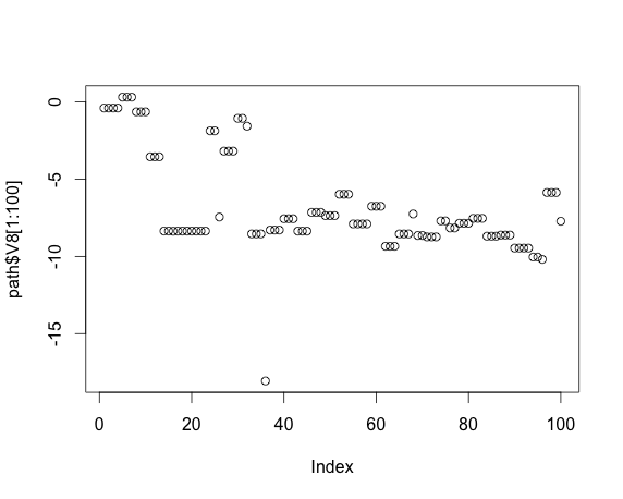

A few other issues we have with this data are that column one is really the timestamp but it comes in as a character. The V3 field is really an artifact of having a double delimiter where the optional sensor values appear. We have the same thing with V11 as each line ends with a delimiter. We can just remove these two. We should also give the fields some better names.

library(lubridate)
# There are two semi colons in a row 
  path$V3 <- NULL
  # The line ends with a semi colon
  path$V11 <- NULL
  
  names(path) <- c('inc', 'timestamp', 'lat', 'long', 'alt', 'acc', 'x', 'y', 'z')
  
  path$date <- as.Date(substr(path$timestamp, 1, 10))
  path$time <- ymd_hms(path$timestamp)

We should also create an index field, the first field currently is the number of milliseconds from the start time. It is also a good idea to turn everything that should be a number into a number.

loc$ind <- seq(nrow(loc))

isNum <- lapply(c(3:9), function(x) class(path[, x]))
any('character' %in% isNum)

## [1] FALSE

for (i in c(3:9)) {
  path[, i] <- as.numeric(path[, i])
}

path$LatLong <- paste(path$lat, path$long, sep = ':')

str(path)

## 'data.frame':    5967 obs. of  13 variables:
##  $ inc      : int  1269 1290 1311 1332 1353 1374 1395 1416 1437 1458 ...
##  $ timestamp: chr  "2014-08-30_11-59-00.732" "2014-08-30_11-59-01.997" "2014-08-30_11-59-03.233" "2014-08-30_11-59-04.495" ...
##  $ lat      : num  38.9 38.9 38.9 38.9 38.9 ...
##  $ long     : num  -77.1 -77.1 -77.1 -77.1 -77.1 ...
##  $ alt      : num  75 75 75 75 75 75 75 75 75 75 ...
##  $ acc      : num  17 17 17 17 18 18 18 17 17 17 ...
##  $ x        : num  -0.394 -0.394 -0.394 -0.394 0.311 0.311 0.311 -0.641 -0.641 -0.641 ...
##  $ y        : num  3.09 3.09 3.09 3.09 1.45 ...
##  $ z        : num  8.95 8.95 8.95 8.95 9.77 ...
##  $ date     : Date, format: "2014-08-30" "2014-08-30" ...
##  $ time     : POSIXct, format: "2014-08-30 11:59:00" "2014-08-30 11:59:01" ...
##  $ ind      : int  1 2 3 4 5 6 7 8 9 10 ...
##  $ LatLong  : chr  "38.949867:-77.082375" "38.949867:-77.082375" "38.949867:-77.082375" "38.949867:-77.082375" ...

It is also a really good idea to put all of this into one function that can read log files and clean them in one step.

read.log <- function(log) {
  firstLine <- readLines(log, 1)
  skip <- if ( firstLine == "--- LOG START  --- ") 1 else 0
  # These are seperated by semicolons and skip one becuase the first line
  # says log output.
  path <- read.csv(log, sep = ';', header = F, skip = skip, stringsAsFactors = F)
  
  # There are two semi colons in a row 
  path$V3 <- NULL
  # The line ends with a semi colon
  path$V11 <- NULL
  
  names(path) <- c('inc', 'timestamp', 'lat', 'long', 'alt', 'acc', 'x', 'y', 'z')
  
  path$date <- as.Date(substr(path$timestamp, 1, 10))
  path$time <- ymd_hms(path$timestamp)
  path$ind <- seq(nrow(path))
  
  # These fields should all be numbers.
  for (i in c(3:9)) {
    # Suppress warnings when NA values are introduced.
    suppressWarnings(path[, i] <- as.numeric(path[, i]))
  }
  
  path$LatLong <- paste(path$lat, path$long, sep = ':')
  
  path
}

Before I do anything with the sensor data I really want to look at it on a map.

library(googleVis)

plotGPS <- function(path, v = 10) {
  if (v == -1) v <- nrow(path)
  if (v > nrow(path)) v <- nrow(path)
  nn <- list(LatLong = path$LatLong[1:v], Tip = path$timestamp[1:v])
  
  m <- gvisMap(nn, 'LatLong' , 'Tip',
               options=list(showTip=TRUE, showLine=FALSE,
                            enableScrollWheel=TRUE,
                            mapType='hybrid', useMapTypeControl=TRUE,
                            width=800,height=400),
               chartid="Run")
  
  plot(m)
}

path <- read.log('LOG_2014-08-30_11-59-00K330_3-axis_Accelerometer.log')

That looks awesome, but we see a problem if we try to look at the whole path, or really any more than I have here.

plotGPS(path, v = 500)

plotGPS(path, v = 3000)

It looks like there is an upper limit to the number of points I can place on the map. The map looks exactly the same and it is a clear giveaway when it says in the top left corner that some data was truncated. I can down-sample it by doing the following.

plotGPS(path[seq(1, 5800, 16), ], v = 5900)

That is pretty rough though. We can eliminate many rows by just removing points that have the same latitude and longitude, this was a point in time where I was standing still. Now I am starting to think I need more utility functions to process this data though.

newPath <- path[!duplicated(path$LatLong), ]
plotGPS(newPath[seq(1, 1625, 8), ], v = -1)