Tacit Web Crawlers

Tacit Programming

Like all paradigms of programming there is no way to say some peece of code is representative or not of the given type. Some peice may be more functional than another or less object oriented than another but in both cases, both could be valid of the respective paradigm. This is partly because the paradigms do not offer strict guidance, which may not be bad, as to what conform and what does not.

Tacit programming or point-free programming is similar, it roughly means that functions do not explicitly refer to arguments. The first question this should raise would be whether this is in realtion to function definition, function usage, or function composition. I think it could mean all three. I have written a lot of code to crawl and scrape data from webpages. I have really come to like using magrittr pipes and rvest for such tasks. Over time I seemed to develop a paradigm that I think is tacit programming. Here are a few more resources about tacit programming.

The following code is the part about function definition. The input argument is never mentioned. I can tell from either the first function that is being composed like in the case of read_html, that this takes in a url, but this information is also contained in the function name. You never really say how that input argument is used.

# Function to take a url and return all of its links.
. %>% read_html %>% html_nodes('a') %>% html_attr('href') -> url_2_links

This may not be real tacit programming because I am using subsequent arguments to later functions but the way Wikipedia states Unix pipes are a type of tacit programming it seems this would be as well.

# get the tags for each 
. %>% html_nodes('.characteristic') %>% 
  html_text %>% grep(':', ., value = T, invert = T) -> get_tag

# and the number of stars
. %>% html_nodes('.star') %>% html_text -> get_score

# and the type of 
. %>% html_nodes('.inside-box') %>% .[2] %>% 
  html_text %>% 
  str_split('Dog Breed Group: ') %>% { .[[1]][2] } %>% 
  str_split('Height: ') %>% { .[[1]][1] } -> get_type

# turn the breed page into a tibble
. %>% read_html %>% 
  { tibble(  tag = get_tag(.), 
           score = get_score(.),
            type = get_type(.) ) } -> url_2_data

If it was not clear we are collecting info about dog breeds. Now we can run these functions to collect the data.

'http://dogtime.com/dog-breeds/groups/' %>% 
  url_2_links %>% 
  grep('breeds/', ., value = T) %>% 
  grep('dog-breeds/groups/', ., value = T, invert = T) -> breeds

So that essentially did some web crawling and scraping, and filtered out the items for which we do not have any interest. Now we can use the map function to turn each URL into data, or a tibble.

breeds %>% map(url_2_data) -> df

df[[1]]

## # A tibble: 31 x 3
##                                tag score           type
##                              <chr> <chr>          <chr>
##  1                    Adaptability       Companion Dogs
##  2 Adapts Well to Apartment Living     5 Companion Dogs
##  3          Good For Novice Owners     4 Companion Dogs
##  4               Sensitivity Level     3 Companion Dogs
##  5           Tolerates Being Alone     1 Companion Dogs
##  6          Tolerates Cold Weather     3 Companion Dogs
##  7           Tolerates Hot Weather     3 Companion Dogs
##  8         All Around Friendliness       Companion Dogs
##  9        Affectionate with Family     5 Companion Dogs
## 10    Incredibly Kid Friendly Dogs     1 Companion Dogs
## # ... with 21 more rows

I think a lot of people I have worked with at first see code like this and think it looks odd, which it might if you are not used to it. I have noticed though that I can come back to web crawling/scraping code that is written in this format after not seeing it for a while and I can easily discern what is happening. Other idioms I have used have always forced me to look back at some of the actual pages and relearn what was trying to happen, it almost reminded me of writing perl code.

The following is an ugly way to add the breed info into each item in the list.

breed <- breeds %>% str_split('/') %>% map_chr(tail, 1)

for (i in 1:length(df)) df[[i]]$breed <- breed[i]

Now we can turn the list of tibbles into just one piece of data. We can also remove the items where that do not have scores, which are the high-level groups. This data is also in a tall format, we can use spread to put it into a wide format so that each dog breed has each characteristic as a variable.

df %>% bind_rows %>% 
  filter(score != ' ') %>% 
  mutate(score = as.numeric(score)) %>%
  spread(key = tag, value = score) -> df

There a few other odds and ends that could be cleaned up as well.

# The names are pretty rough.
df %>% set_names(c(names(.)[1:2], paste0('x', 1:(ncol(.)-2)))) -> df

# Remove mutts, hybrids and NA's
df %>% filter(breed != 'mutt', type != 'Hybrid Dogs') %>% na.omit -> dfx

I wonder if these were made in a way that similar breeds fall into the same group. Could either supervised or unsupervised learning shed some light on this. If a supervised model could predict a holdout set or if an unsupervised model placed them all into the same group it could add some strength this.

First we can try a supervised approach.

dfx %>% group_by(type) %>% mutate(obs = row_number()) -> dfx

train <- dfx %>% filter(obs <= 25) 
test <- dfx %>% filter(obs > 25) 
  
mod <- randomForest(factor(type) ~ ., data = select(train, -breed, -obs))

test$pred <- as.character(predict(mod, newdata = test))

sum(test$type == test$pred)

## [1] 19

sum(test$type != test$pred)

## [1] 17

Not great, let’s try unsupervised.

dfx %>% select(type, breed, obs, everything()) -> dfx

a <- kmeans(dfx[, -c(1:3)], 6)

dfx$clus <- a$cluster
table(dfx$type, dfx$clus)

##                 
##                   1  2  3  4  5  6
##   Companion Dogs  9  1 14 11  0  1
##   Herding Dogs    1 10  0  8  1  8
##   Hound Dogs     10  2  4  1  1 13
##   Sporting Dogs   2  4  1  4  1 21
##   Terrier Dogs    6  8  2  7  1  2
##   Working Dogs    2  3  1  1 17  8

A little bit more coherent. Perhaps there are just too many variables. We can do a quick bit of dimensionality reduction.

dfx$clus <- NULL
dfx %>% select(type, breed, obs, everything()) -> dfx

b <- prcomp(dfx[, -c(1:4)])
screeplot(b)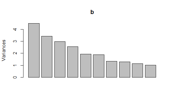

dfx %>% select(type, breed, obs) %>% bind_cols(as_tibble(b$x[, 1:5])) -> dfx2 

train <- dfx2 %>% filter(obs <= 25) %>% select(-breed, -obs)
test <- dfx2 %>% filter(obs > 25) 
  
mod <- randomForest(factor(type) ~ ., data = train, ntree = 1000)

test$pred <- as.character(predict(mod, newdata = test))

sum(test$type == test$pred)

## [1] 15

sum(test$type != test$pred)

## [1] 21

c <- kmeans(b$x[, 1:5], 6)

dfx$clus <- c$cluster
table(dfx$type, dfx$clus)

##                 
##                   1  2  3  4  5  6
##   Companion Dogs  3  0 15  7  8  3
##   Herding Dogs    1  1  0 13  6  7
##   Hound Dogs     17  0  2  3  2  7
##   Sporting Dogs   8  0  0  6  4 15
##   Terrier Dogs    3  1  2  9  3  8
##   Working Dogs    2 18  0  4  1  7

The supervised method seemed to work far worse while the unsupervised seems to be a little better. That last statement is also far from precise or rigorous. I really wanted to talk about rvest, web crawling and scraping and tacit programming. The last bit was just a rough method to discern something about the grouping of dog breeds. I bet I could spend more effort and be able to predict them or group them better but I think one of two things is happening. It is possible there is a strict method to group them but these features are more useful for people looking into acquiring a dog. It is also possible that the groupings are not coherent so the methods to group them is more subjective. I have used this approach before as a method to determine whether there is a latent rule under some data and when I know there is it does seem to work, so long as the latent rule is not overly complicated. Still a random forest would be the thing to root out complicated.