How would you determine who is the best three-point shooter in the NBA? Is it the same as the best two point-shooter or the best free throw shooter. There is a three-point competition but that is a little different from what this question is asking. One of two next steps are commonly pursued to answer a question of this sort. Each has its own pitfalls. By trying to answer this question we can see how both of them fall apart.
We will use some NBA player statistics. It is basically the season totals for each player. Here is roughly what it looks like.
head(details)## Source: local data frame [6 x 14]
##
## name birth season three_made three_attempt two_made
## (chr) (chr) (chr) (dbl) (dbl) (dbl)
## 1 Alaa Abdelnaby June 24, 1968 1990-91 0 0 55
## 2 Alaa Abdelnaby June 24, 1968 1991-92 0 0 178
## 3 Alaa Abdelnaby June 24, 1968 1992-93 0 1 245
## 4 Alaa Abdelnaby June 24, 1968 1992-93 0 1 26
## 5 Alaa Abdelnaby June 24, 1968 1992-93 0 0 219
## 6 Alaa Abdelnaby June 24, 1968 1993-94 0 0 24
## Variables not shown: two_attempt (dbl), ft_made (dbl), ft_attempt (dbl),
## rebounds (dbl), assist (dbl), steal (dbl), block (dbl), turnover (dbl)For the first method, we are going to calculate the average, that is shots made divided by attempts. First we will focus on just three-point shooting. We first group by player, which is uniquely defined by the name and birthday, then we sum over the number of shots made and attempted. We then divide the total number of shots made by the total number shots attempted. If we then sort on the average we should be able to see who is the best three-point shooter?
details %>%
  group_by(name, birth) %>%
  summarise(three_made = sum(three_made),
            three_attempt = sum(three_attempt)) %>%
  select(-birth) %>%
  ungroup %>%
  mutate(three_avg = three_made / three_attempt) %>%
  arrange(desc(three_avg)) -> threes

head(threes)
## Source: local data frame [6 x 4]
##
## name three_made three_attempt three_avg
## (chr) (dbl) (dbl) (dbl)
## 1 Al Salvadori 1 1 1
## 2 Alvin Sims 1 1 1
## 3 Bill Allen 2 2 1
## 4 Carroll Hooser 1 1 1
## 5 Coty Clarke 2 2 1
## 6 David Gaines 1 1 1Clearly this did not work. This method is obviously flawed since we know the best three-point shooters should have taken more than only a couple of shots. These are really just people that only made a few attempts, they may be good but they may also just be lucky.
threes %>% filter(three_avg == 1) %>%
  arrange(desc(three_made))
## Source: local data frame [21 x 4]
##
## name three_made three_attempt three_avg
## (chr) (dbl) (dbl) (dbl)
## 1 Gundars Vetra 3 3 1
## 2 Bill Allen 2 2 1
## 3 Coty Clarke 2 2 1
## 4 Eddy Curry 2 2 1
## 5 Eric Anderson 2 2 1
## 6 Al Salvadori 1 1 1
## 7 Alvin Sims 1 1 1
## 8 Carroll Hooser 1 1 1
## 9 David Gaines 1 1 1
## 10 Eric White 1 1 1
## .. ... ... ... ...We can also see what would be the result if we were to ask the question who is the worst three-point shooter. This method produces just as bad of an error.
threes %>% filter(three_avg == 0) %>%
  arrange(desc(three_made))
## Source: local data frame [480 x 4]
##
## name three_made three_attempt three_avg
## (chr) (dbl) (dbl) (dbl)
## 1 A.J. Wynder 0 1 0
## 2 Aaron Gray 0 4 0
## 3 Abdul Jeelani 0 7 0
## 4 Acie Earl 0 14 0
## 5 Adonal Foyle 0 2 0
## 6 Adrian Caldwell 0 5 0
## 7 Alaa Abdelnaby 0 6 0
## 8 Alan Hardy 0 5 0
## 9 Alan Ogg 0 2 0
## 10 Alex Blackwell 0 3 0
## .. ... ... ... ...So this method does not work. There has been a lot of discussion of this problem. It is talked about in the book Thinking Fast and Slow. There is a very interesting example of rural counties having both the highest and lowest cancer rates, one dicsussion of that can be found here. What is happening is that in the cases with fewer observations have more room for variance, thus just a few flips in either direction will really skew things. As a player takes more shots the average will start to approach the true average. We can see that effect here in this plot.
threes %>%
  ggplot(aes(three_attempt, three_avg)) +
  geom_point() +
  geom_smooth(method = "lm", se = FALSE) +
  scale_x_log10()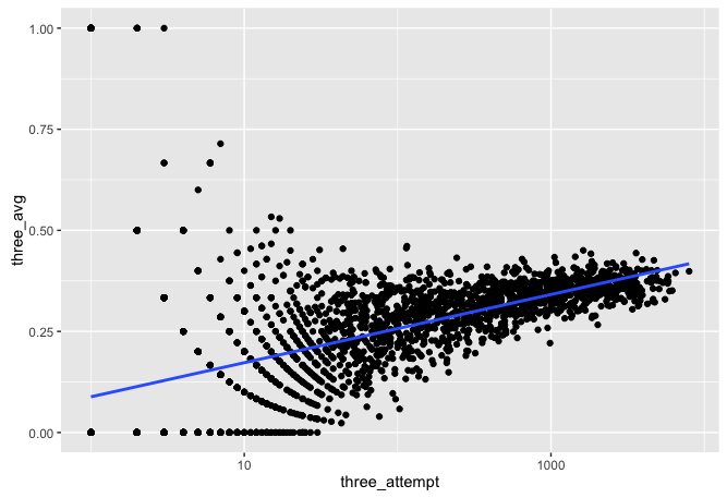
What if we just looked at it by who made the most?
threes %>% arrange(desc(three_made)) %>% head## Source: local data frame [6 x 4]
##
## name three_made three_attempt three_avg
## (chr) (dbl) (dbl) (dbl)
## 1 Ray Allen 3174 7962 0.3986436
## 2 Reggie Miller 2560 6486 0.3946963
## 3 Chauncey Billups 2245 5810 0.3864028
## 4 Vince Carter 2180 5823 0.3743775
## 5 Jason Terry 2169 5724 0.3789308
## 6 Jason Kidd 2168 6178 0.3509226This may look more valid but Jason Terry made one more than Jason Kidd but it took 454 less tries also. Vince Carter made eleven more shots than Jason Terry but he also took 99 more shots. Since Jason Terry has an average of around 37% if he was to take 99 more shots he would most likely have made at least eleven of them.
To get over this issue we can use what is known as Empirical Bayes Estimation. You can see the inspirational example here What this method does is that it creates a baseline for the distribution and then adjusts it based on the number of shots made and attempted.
We need to fit a beta distribution to our data. But first we need to remove some of the crazy observations so as to not taint the empirical prior.
threes %>%
  filter(three_attempt >= 500) -> three_filt

m <- suppressWarnings(MASS::fitdistr(three_filt$three_avg, dbeta,
                    start = list(shape1 = 1, shape2 = 10)))

(alpha0 <- m$estimate[1])
## shape1
## 64.37282(beta0 <- m$estimate[2])## shape2
## 119.3305ggplot(three_filt) +
geom_histogram(aes(three_avg, y = ..density..), binwidth = .005) +
stat_function(fun = function(x) dbeta(x, alpha0, beta0), color = "red", size = 1) +
xlab("Three Point Percentage")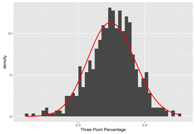
Now to construct the new estimate using the players' data and this beta distribution we apply a couple of additions.
threes %>%
  filter(three_attempt > 0) %>%
  mutate(est = (three_made + alpha0) / (three_attempt + alpha0 + beta0)) -> threes
And now we can see more practical results.
threes %>% arrange(est) %>% head## Source: local data frame [6 x 5]
##
## name three_made three_attempt three_avg est
## (chr) (dbl) (dbl) (dbl) (dbl)
## 1 Andre Miller 218 986 0.22109533 0.2414055
## 2 Avery Johnson 32 215 0.14883721 0.2417156
## 3 Darrell Walker 6 103 0.05825243 0.2454552
## 4 Kelvin Ransey 20 152 0.13157895 0.2513315
## 5 Darwin Cook 63 321 0.19626168 0.2523717
## 6 Speedy Claxton 53 279 0.18996416 0.2536676threes %>% arrange(est) %>% tail## Source: local data frame [6 x 5]
##
## name three_made three_attempt three_avg est
## (chr) (dbl) (dbl) (dbl) (dbl)
## 1 Kyle Korver 1998 4691 0.4259220 0.4230766
## 2 Steve Nash 1685 3939 0.4277735 0.4243266
## 3 Steve Novak 626 1440 0.4347222 0.4251841
## 4 Hubert Davis 806 1823 0.4421284 0.4337327
## 5 Stephen Curry 1593 3590 0.4437326 0.4391900
## 6 Steve Kerr 732 1625 0.4504615 0.4403004This plot is also borrowed from the above mentioned blog. It does a great job at showing the shrinkage to baseline. When you have very shots attempted you are pulled further to the mean. Points are pulled down if they are above and pulled up if they are below. The amount of the pull depends on the number of shots, so the lighter blue do not get shrunken nearly as much.
ggplot(threes, aes(three_avg, est, color = three_attempt)) +
  geom_hline(yintercept = alpha0 / (alpha0 + beta0), color = "red", lty = 2) +
  geom_point() +
  geom_abline(color = "red") +
  scale_colour_gradient(trans = "log", breaks = 10 ^ (1:5)) +
  xlab("Field Goal Percentage") +
  ylab("Empirical Bayes Field Goal Percentage")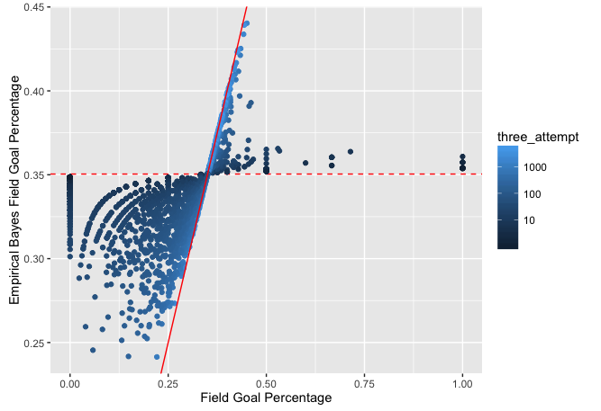
Some issues to think about here though. If you were pretty bad in first few games, you may not play for long. We may also see some impact from players who stayed in the NBA beyond there prime. Thus at one point in there career they may have been the best ever, but earlier and later seasons may weaken this. We could try to get around this by asking what is the best season average.
details %>%
  select(name, birth,
         three_made, three_attempt, season) -> threes_season
head(threes_season)
## Source: local data frame [6 x 5]
##
## name birth three_made three_attempt season
## (chr) (chr) (dbl) (dbl) (chr)
## 1 Alaa Abdelnaby June 24, 1968 0 0 1990-91
## 2 Alaa Abdelnaby June 24, 1968 0 0 1991-92
## 3 Alaa Abdelnaby June 24, 1968 0 1 1992-93
## 4 Alaa Abdelnaby June 24, 1968 0 1 1992-93
## 5 Alaa Abdelnaby June 24, 1968 0 0 1992-93
## 6 Alaa Abdelnaby June 24, 1968 0 0 1993-94threes_season %>%
group_by(name, birth, season) %>%
summarise(three_made = sum(three_made), three_attempt = sum(three_attempt)) %>%
ungroup %>%
filter(three_attempt > 0) %>%
mutate(three_avg = three_made / three_attempt) %>%
arrange(desc(three_avg)) -> threes_season
threes_season %>%
ggplot(aes(three_attempt, three_avg)) +
geom_point() +
geom_smooth(method = "lm", se = FALSE) +
scale_x_log10()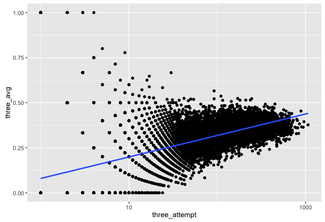
This is very similar
threes_season %>%
  filter(three_attempt >= 200) -> threes_season_filt

m <- suppressWarnings(MASS::fitdistr(threes_season_filt$three_avg, dbeta,
                                     start = list(shape1 = 1, shape2 = 10)))

alpha0 <- m$estimate[1]
beta0 <- m$estimate[2]

ggplot(threes_season_filt) +
  geom_histogram(aes(three_avg, y = ..density..), binwidth = .005) +
  stat_function(fun = function(x) dbeta(x, alpha0, beta0), color = "red", size = 1) +
  xlab("Seasonal Three Point Percentage")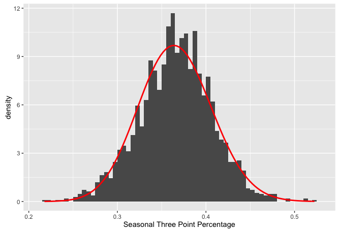
threes_season %>%
   filter(three_attempt > 0) %>%
  mutate(est = (three_made + alpha0) / (three_attempt + alpha0 + beta0)) -> threes_season

threes_season %>% select(-birth) -> threes_season


threes_season %>% arrange(desc(est)) %>% select(-three_made, -three_attempt) %>% head(20)
## Source: local data frame [20 x 4]
##
## name season three_avg est
## (chr) (chr) (dbl) (dbl)
## 1 Tim Legler 1995-96 0.5224490 0.4662383
## 2 Kyle Korver 2014-15 ★ 0.4922049 0.4626337
## 3 Steve Kerr 1995-96 0.5147679 0.4601699
## 4 Craig Hodges 1987-88 0.4914286 0.4560655
## 5 Jason Kapono 2006-07 0.5142857 0.4556309
## 6 Steve Kerr 1994-95 0.5235294 0.4531079
## 7 Detlef Schrempf 1994-95 ★ 0.5138122 0.4500138
## 8 J.J. Redick 2015-16 0.4750594 0.4482160
## 9 Joe Johnson 2004-05 0.4783784 0.4479380
## 10 Steve Novak 2010-11 0.5652174 0.4458721
## 11 Dale Ellis 1988-89 ★ 0.4778761 0.4455982
## 12 Glen Rice 1996-97 ★ 0.4704545 0.4455888
## 13 Kyle Korver 2013-14 0.4719388 0.4444326
## 14 Jose Calderon 2012-13 0.4609929 0.4423752
## 15 Steve Nash 2007-08 ★ 0.4698163 0.4422877
## 16 Stephen Curry 2015-16 ★ 0.4537246 0.4419404
## 17 Kyle Korver 2009-10 0.5363636 0.4417209
## 18 Dana Barros 1994-95 ★ 0.4635294 0.4396890
## 19 Hubert Davis 1995-96 0.4756554 0.4383795
## 20 Steve Kerr 1989-90 0.5069444 0.4380973It is a little reassuring to see the stars next to the season which indicates that this player was an all star that year.
ggplot(threes_season, aes(three_avg, est, color = three_attempt)) +
  geom_hline(yintercept = alpha0 / (alpha0 + beta0), color = "red", lty = 2) +
  geom_point() +
  geom_abline(color = "red") +
  scale_colour_gradient(trans = "log", breaks = 10 ^ (1:5)) +
  xlab("Seasonal Three Point Percentage") +
  ylab("Empirical Bayes Seasonal Three Point Percentage")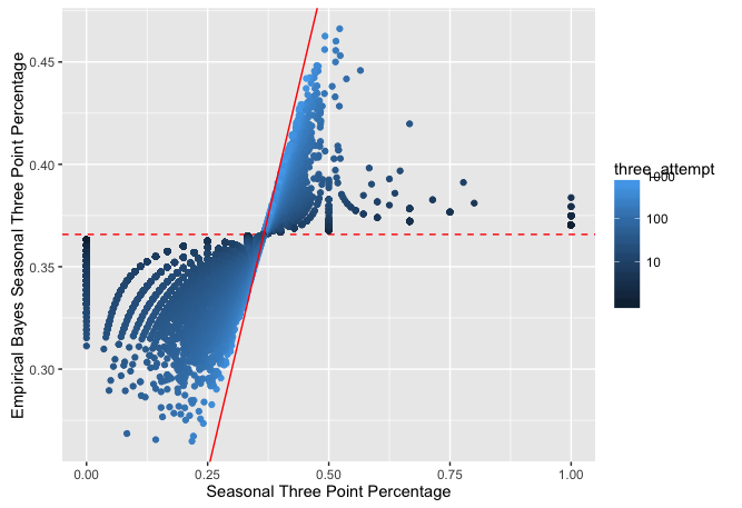
Another interesting thing to do is apply this to free throws and two pointers.
details %>%
  group_by(name, birth) %>%
  summarise(two_made = sum(two_made),
            two_attempt = sum(two_attempt),
            ft_made = sum(ft_made),
            ft_attempt = sum(ft_attempt)) %>%
  select(-birth) %>% ungroup -> totals

head(totals)
## Source: local data frame [6 x 5]
##
## name two_made two_attempt ft_made ft_attempt
## (chr) (dbl) (dbl) (dbl) (dbl)
## 1 A.C. Green 4653 9177 3247 4447
## 2 A.J. Bramlett 4 21 0 0
## 3 A.J. English 608 1353 259 333
## 4 A.J. Guyton 93 247 37 45
## 5 A.J. Price 367 834 223 303
## 6 A.J. Wynder 3 11 6 8totals %>%
mutate(two_avg = two_made / two_attempt,
ft_avg = ft_made / ft_attempt) -> totalsIt is very interesting to note that we see the same effect but it is just shifted around this shot types true mean.
totals %>%
  ggplot(aes(ft_attempt, ft_avg)) +
  geom_point() +
  geom_smooth(method = "lm", se = FALSE) +
  scale_x_log10()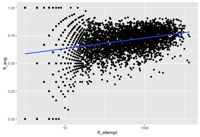
totals %>%
  ggplot(aes(two_attempt, two_avg)) +
  geom_point() +
  geom_smooth(method = "lm", se = FALSE) +
  scale_x_log10()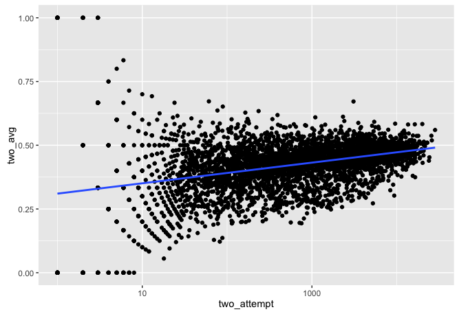
totals %>% filter(ft_attempt >= 1000) -> filt1
totals %>% filter(two_attempt >= 1000) -> filt2

m1 <- suppressWarnings(MASS::fitdistr(filt1$ft_avg, dbeta,
                    start = list(shape1 = 1, shape2 = 10)))
m2 <- suppressWarnings(MASS::fitdistr(filt2$two_avg, dbeta,
                    start = list(shape1 = 1, shape2 = 10)))


totals %>%
  mutate(est_1 = (ft_made + m1$estimate[1]) /
           (ft_attempt + m1$estimate[1] + m1$estimate[2]),
         est_2 = (two_made + m2$estimate[1]) /
           (two_attempt + m2$estimate[1] + m2$estimate[2])) %>% na.omit %>% ungroup -> totals

totals %>% select(name, ft_made, ft_attempt, est_1) %>% arrange(desc(est_1)) %>% head
## Source: local data frame [6 x 4]
##
## name ft_made ft_attempt est_1
## (chr) (dbl) (dbl) (dbl)
## 1 Steve Nash 3060 3384 0.9027327
## 2 Mark Price 2135 2362 0.9017280
## 3 Mahmoud Abdul-Rauf 1051 1161 0.9008704
## 4 Brian Roberts 345 378 0.8993686
## 5 Stephen Curry 1668 1850 0.8989065
## 6 Peja Stojakovic 2498 2785 0.8951895totals %>% select(name, two_made, two_attempt, est_2) %>% arrange(desc(est_2)) %>% head## Source: local data frame [6 x 4]
##
## name two_made two_attempt est_2
## (chr) (dbl) (dbl) (dbl)
## 1 DeAndre Jordan 2074 3088 0.6662031
## 2 Brandan Wright 1422 2324 0.6066962
## 3 Hassan Whiteside 668 1096 0.5990589
## 4 Greg Smith 243 393 0.5908849
## 5 Andris Biedrins 1432 2407 0.5904658
## 6 Tyson Chandler 3209 5422 0.5898742It is interesting that we see Stephen Curry in a couple of all nut one of these tables. This brings up the question of who is the best all overall shooter? Or even more interesting who is the best overall player. I want to cover that next, but that is a task for another day.