Getting Setup With Spark

Motivating Example

To get started, a motivating example. Flight data from roughly 20 years.

options(stringsAsFactors = FALSE)
library(dplyr)
library(lubridate)

system.time(f <- read.csv('2008.csv'))

##    user  system elapsed 
##   112.552   2.115 114.649

# How big is this 
format(object.size(f), units = "auto")

## [1] "909.4 Mb"

This dataset is pretty large but we can still work with the data fairly quickly once it is loaded into RAM.

system.time(f %>% group_by(Origin) %>%
  summarize(incoming = n()) %>%
  rename(airport = Origin) -> inbound) 

##    user  system elapsed 
##   0.228   0.069   0.296

system.time(f %>% group_by(Dest) %>%
  summarize(outgoing = n()) %>%
  rename(airport = Dest) %>%
  inner_join(inbound, by = 'airport') %>%
  mutate(delta = incoming - outgoing) %>%
  mutate(diff = abs(delta)) %>%
  arrange(desc(diff)) -> flights)

##    user  system elapsed 
##   0.237   0.029   0.266

Once we get the data loaded into RAM working with it is not that bad, but the challenge is getting into RAM.

I have never been able to get this plot to run. It is just to many observations for my machine!

plot(f$DepTime, f$ArrTime)

This plot will take forever and most likely crash!

A few notes so far:

• One year of data is roughly one gigabyte of RAM
• We can do some analysis on this data
• It will be very slow to make plots

So what if we wanted to scale this up to all 22 years or more? It may work on some machines, but they would need to be powerful! What about if we had 100 years of data? What if we have more info on every flight? Having a more powerful machine is not that compelling of an option!

We could load all year like this. For most people this wont work, your machine will just bog down as it asymptotically fills your RAM.

f <- list()
data <- list.files(pattern = 'csv')[1:22]
for (i in data) {
  f[[i]] <- read.csv(i)
  print(i)
  print(format(object.size(f), units = "auto"))
}

What are our options? Is this where sampling comes into play? What if our goal was to find the page rank of each airport? Sampling works well in some cases and it others it is not valid. We can’t just sample a network, we could sample and get the average flights for day but not the Pagerank!

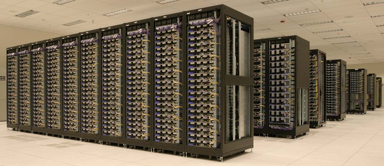
• Getting a bigger more powerful machine has been the historic approach
• Companies have bought bought bigger more powerful servers for years, but the are expensive.

Will this always work?

• What if data collection continues to grow and next year this server fails?
• I have to buy another one, then another. It does not scale.
• If this is too expensive to get a bigger more powerful machine are there other options?

Advanced Computing

There are three different methods which I would consider advanced computing.

Apache Hadoop to the Rescue

Instead of trying to explain Hadoop and where it came from I will leave that to the expert. In the The Evolution of the Apache Hadoop Ecosystem Doug Cutting explains where Hadoop came from. In The Apache Hadoop Ecosystem he describes why it came to be.

Problem Solved

• So we need distributed computing
• We have Hadoop
• Problem solved

Not so fast

• The first iteration of ‘Big Data’ was confusing
• Everybody spoke about Hadoop and how great it was
• They were not wrong, it did make all sorts of things possible
• But many didn’t quite understood what it was, and they still probably do not.

To effectively use Hadoop …

• An expert in Linux
• Plenty of knowledge of ETL and data processing skills
• Expert in Java, which is object oriented, but mapreduce is functional,
• You need to understand hardware
• Knowledge of distributed systems.

Who understands this and knows how to use data? Nobody, well very few at least.

The people who actually use data to solve problems have two large issues to overcome.

Problem 1 - You have to write mapreduce code.

Problem 2 - You have to actually setup a cluster.

Thus Hadoop may not be the solution!

• Hadoop is so 2012
• Data Scientists should not be writing code for Hadoop
• The ecosystem is changing very frequently to resolve this issue
• History

And then there was Spark

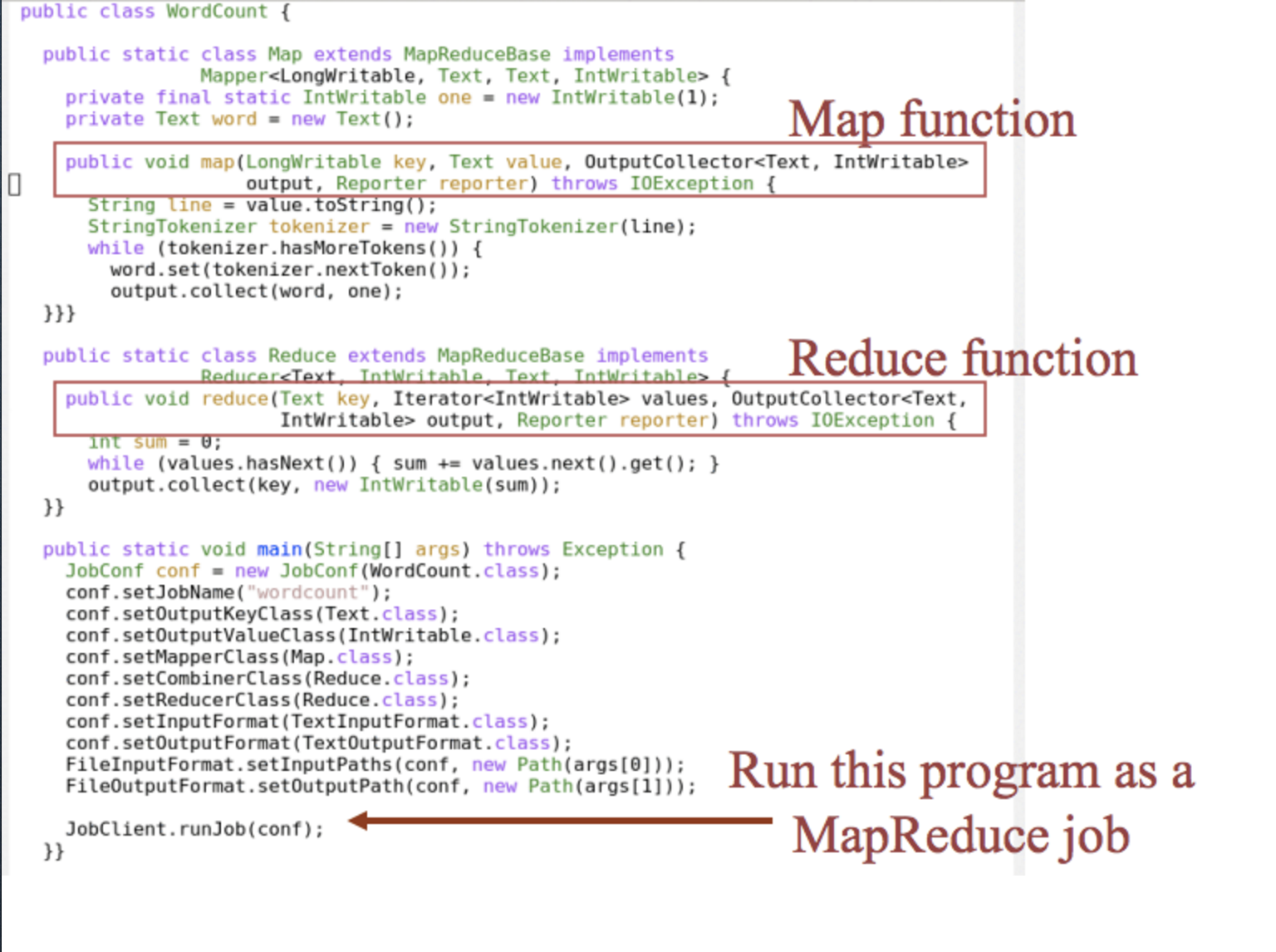
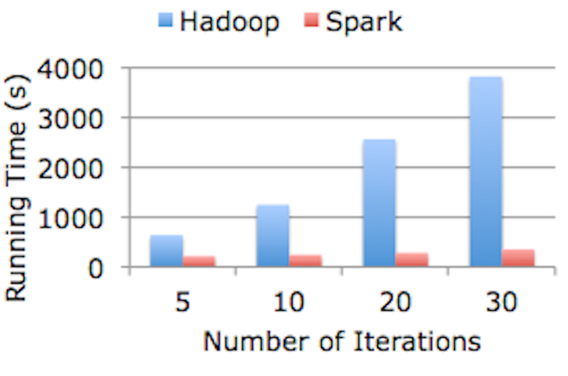
Remember the mapreduce code. This is what mapreduce code looks like

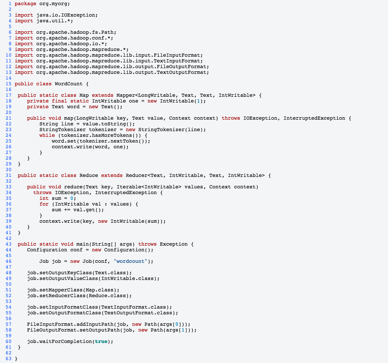
This is the equivalent code in Spark

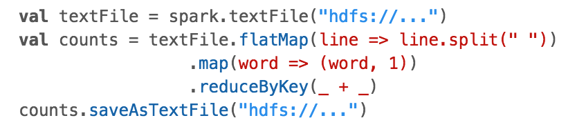
It is also much faster!

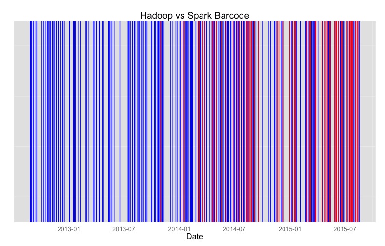
So Hadoop is old news. If that did not convince you maybe this will. This is a collection of job posting. Each blue line is a job that mentions Hadoop while each red line mentions Spark.

Today

• Spark came along and got rid of the need to be an expert Java programmer.
• Thus we may be able to say we have solved problem number 1.

Spark Ecosystem

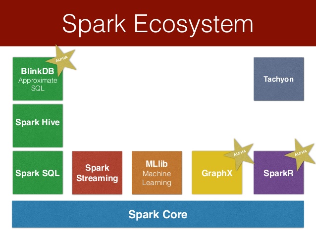
This all makes Spark a hit

Spark is a hit for data science!

Using Spark

If you do some looking around you may find some of these options;

AWS

• Running Spark on AWS
• Using Spark and Jupyter, streaming means
• Spark is a giant tradeoff
• It is usable by data scientists
• It is also usable by software engineers and devops folks
• Non of the above options seem very appealing
• There has to be a better way

Using Spark

We are going to use spark in standalone or local mode

Instructions for Downloading Spark (versions will change)

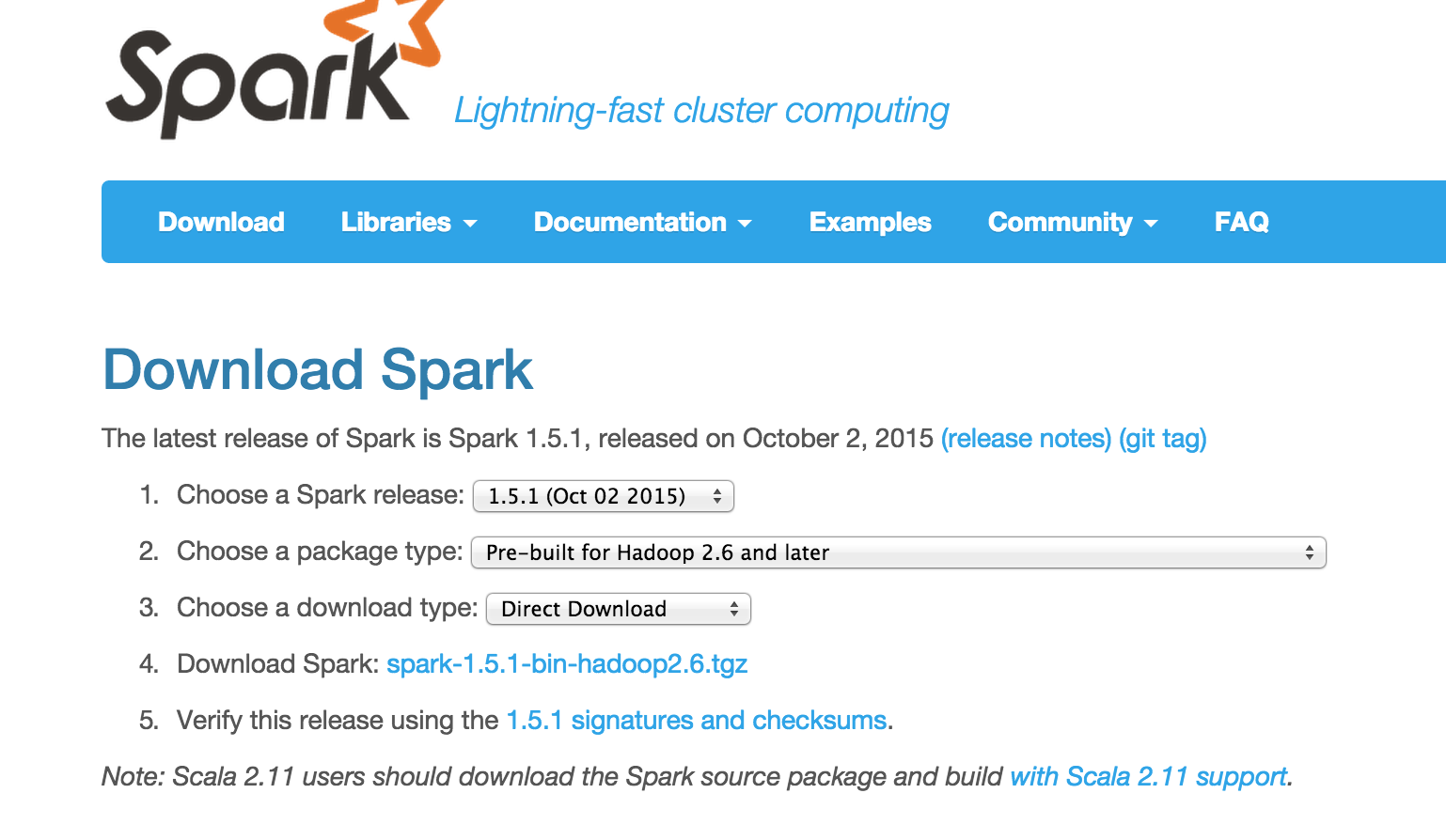
In any browser navigate to the download page

1. For the release type select ‘1.5.1 (Oct 02 2015)’
2. For package type select ‘Pre-built for Hadoop 2.6 and later’
3. For download type select ‘Direct Download’
4. Click the link to download

Unzip the file

On windows use 7zip or

On Mac or Linux run the following in the directory containing the download

tar zxvf spark-1.5.1-bin-hadoop2.6.tgz

What is the difference?

• So far the options are more on the software engineering side
• They let you use Spark in a cluster setting
• Local mode is still constrained by a your machine
• But it is much easier to get setup
• It’s also the exact same

sparkR.init(master="local")

vs

sparkR.init(master="spark://<master>:7077")

Spark API

• We can use sparkr or pyspark just like we would use r or python
• Python option
• R option

For data science

slides on sparkr

Sparkr Command line

./bin/sparkR

sc <- sparkR.init("local")
lines <- SparkR:::textFile(sc, 'index.html')
length(lines)

One major thing to notice here is that you must use three semicolons. This is strange because you just loaded the package but many of its contents are not exported to the workspace. Hopefully this will go away in the future. Next to make things really useful you may want to work somewhere other than in the command line. We can get spark running in RStudio by doing the following from with RStudio.

Sys.setenv(SPARK_HOME = '/Users/kdarrell/Desktop/Spark-1.5.1')

.libPaths(c(file.path(Sys.getenv("SPARK_HOME"), "R", "lib"), .libPaths()))

# Make sure you don't have spark from CRAN!
library(SparkR)

Launching java with spark-submit command /Users/kdarrell/Desktop/Spark-1.5.1/bin/spark-submit   sparkr-shell /var/folders/kc/668j7hpn135fvf8b96gctp5c0000gp/T//RtmpzqTVUG/backend_port6ee75eafa8e4 
16/02/07 10:43:02 WARN NativeCodeLoader: Unable to load native-hadoop library for your platform... using builtin-java classes where applicable
16/02/07 10:43:03 WARN MetricsSystem: Using default name DAGScheduler for source because spark.app.id is not set.

sc <- sparkR.init("local")

lines <- SparkR:::textFile(sc, 'index.html')
length(lines)

##  [1] 781

You may see an awful lot of output messages. You need to turn log options to a less verbose setting. To do this make a copy of the following file, just removing template from the name.

conf/log4j.properties.template

conf/log4j.properties

Inside of this new file you need to make one change. Locate the as seen below and replace INFO with WARN.

log4j.rootCategory=INFO, console

With this

log4j.rootCategory=WARN, console

What all can we do in Spark?

For access to data.frames we need Spark SQL

sqlContext <- sparkRSQL.init(sc)

df <- createDataFrame(sqlContext, faithful) 

Is it really the same?

head(faithful)

  eruptions waiting
1     3.600      79
2     1.800      54
3     3.333      74
4     2.283      62
5     4.533      85
6     2.883      55

head(df)

  eruptions waiting
1     3.600      79
2     1.800      54
3     3.333      74
4     2.283      62
5     4.533      85
6     2.883      55

Which looks the same.

faithful$eruptions

  [1] 3.600 1.800 3.333 2.283 4.533 2.883 4.700 3.600 1.950
 [10] 4.350 1.833 3.917 4.200 1.750 4.700 2.167 1.750 4.800

df$eruptions

  Column eruptions

This looks a little different though!

faithful[1, ]

  eruptions waiting
1       3.6      79

df[1, ]

Error in df[1, ] : object of type 'S4' is not subsettable

It is strange that this does not work.

lm(faithful$eruptions ~ faithful$waiting)

Call:
lm(formula = faithful$eruptions ~ faithful$waiting)

Coefficients:
     (Intercept)  faithful$waiting  
        -1.87402           0.07563  

lm(df$eruptions ~ df$waiting)

Error in model.frame.default(formula = df$eruptions ~ df$waiting, drop.unused.levels = TRUE) : 
  object is not a matrix

So have we lost all of the great things we can do in R. In some ways yes, but not really. We can now use Spark where it makes sense, then for things that Spark can't do we use base R by pulling the data out of Spark. We also have to realize when Spark does something different than R. First though, why so many differences? We are not really using R any more! We are using and api to spark inside of R The api is growing to act more like R and support more of its functionality though

So if we want to do machine learning stuff what do we do? We need to use the methods supplied by Spark.

# https://spark.apache.org/docs/latest/sparkr.html#creating-dataframes
# Create the DataFrame
df <- createDataFrame(sqlContext, iris)

Warning messages:
1: In FUN(X[[i]], ...) :
  Use Sepal_Length instead of Sepal.Length  as column name
2: In FUN(X[[i]], ...) :
  Use Sepal_Width instead of Sepal.Width  as column name
3: In FUN(X[[i]], ...) :
  Use Petal_Length instead of Petal.Length  as column name
4: In FUN(X[[i]], ...) :
  Use Petal_Width instead of Petal.Width  as column name

What happened here was that Spark does not like periods in variable names, so it changed them for us. We need to remember that when we work with two different sets of rules.

SparkR::glm

## standardGeneric for "glm" defined from package "stats"
## 
## function (formula, family = gaussian, data, weights, subset, 
##     na.action, start = NULL, etastart, mustart, offset, control = list(...), 
##     model = TRUE, method = "glm.fit", x = FALSE, y = TRUE, contrasts = NULL, 
##     ...) 
## standardGeneric("glm")
## <environment: 0x7f9f8be20630>
## Methods may be defined for arguments: formula, family, data, weights, subset, na.action, start, etastart, mustart, offset, control, model, method, x, y, contrasts
## Use  showMethods("glm")  for currently available ones.

stats::glm

## function (formula, family = gaussian, data, weights, subset, 
##     na.action, start = NULL, etastart, mustart, offset, control = list(...), 
##     model = TRUE, method = "glm.fit", x = FALSE, y = TRUE, contrasts = NULL, 
##     ...) 
## {
##     call <- match.call()
##     if (is.character(family)) 
##         family <- get(family, mode = "function", envir = parent.frame())
##     if (is.function(family)) 
##         family <- family()
##     if (is.null(family$family)) {
## ...
## ...
## ...
## }
## <bytecode: 0x7f9f8bde02b0>
## <environment: namespace:stats>

Use this to fit a linear model over the dataset.

model <- glm(Sepal_Length ~ Sepal_Width + Species, data = df, family = "gaussian")

summary(model)

$coefficients
                     Estimate
(Intercept)         2.2513930
Sepal_Width         0.8035609
Species__versicolor 1.4587432
Species__virginica  1.9468169

predictions <- predict(model, newData = df)
head(select(predictions, "Sepal_Length", "prediction"))

  Sepal_Length prediction
1          5.1   5.063856
2          4.9   4.662076
3          4.7   4.822788
4          4.6   4.742432
5          5.0   5.144212
6          5.4   5.385281

Back to the flight data. Can we now read the CSV in from earlier?

# First thought
df <- createDataFrame(sqlContext, read.csv('2008.csv'))

# Second thought
df <- read.df(sqlContext, '2008.csv', source = "csv")

# Third thought
customSchema <- structType(
    structField("year", "integer"), 
    structField("make", "string"),
    structField("model", "string"),
    structField("comment", "string"),
    structField("blank", "string"))

df <- read.df(sqlContext, "cars.csv", source = "com.databricks.spark.csv", schema = customSchema)

Whats the deal. We can't even load a CSV file. Well if we think more about this problem, is it a big concern if Spark can't do this. If your data exists in a CSV file you could probably get away without needing Spark to being with. But it is useful for working in the local mode to get an understanding of Spark. This functionality is available, just not by default. We need the CSV package. That right, Spark has packages just like R. How do we load them?

From the command line for Scala:

bin/spark-shell --packages com.databricks:spark-csv_2.10:1.0.3

From the command line for R:

bin/sparkR --packages com.databricks:spark-csv_2.10:1.0.3

A few other itmes

# Starting Spark as normal
sc <- sparkR.init("local")
# Stopping our session.
sparkR.stop()
# You can start it with a reference to packages or any other arguments.
Sys.setenv('SPARKR_SUBMIT_ARGS'='"--packages" "com.databricks:spark-csv_2.10:1.2.0" "sparkr-shell"')
sc <- sparkR.init("local")
sparkR.stop()
# You can start it give it more memory.
sc <- sparkR.init("local", sparkEnvir=list(spark.executor.memory="10g"))

Running SQL

faith <- createDataFrame(sqlContext, faithful)

printSchema(faith)

# Register this DataFrame as a table.
registerTempTable(faith, "faith")

# SQL statements can be run by using the sql method
long <- sql(sqlContext, "SELECT * FROM faith WHERE waiting > 50")
head(long)

Everything I have done thus far is for a Mac, or maybe Linux. I did quite a bit of trouble shooting of students issues on Windows and ran into differnt types of issues. On Windows (cross your fingers) you may need this, as it helped me.

Review

This was the start of the seconds lecture.

1. Limitations of systems like R and Python
2. Distributed computing
3. Hadoop/HDFS
4. Spark
5. SparkR
6. API

Limitations of systems like R and Python

R and Python are great for small and medium sized

There are many other (attempted) definitions of these, but for our purpose this one works pretty well. (Thanks to Hadley Wickham)

Small Data - Fits in memory on a laptop: < 10 GB Medium Data - Fits in memory on a server or disk on a laptop: 10 GB - 1 TB Big Data - Can’t fit in memory on any one machine: > 1 TB

R and Python are great for Small Data. They can be good for Medium data if you have a server or with some decent coding chops on a single laptop. They are both terrible at number Big Data, on there own that is.

Distributed computing

Distributed computing was made much easier (not easy just easier) via research by Google that eventually reached open source by the name Hadoop/HDFS.

Distributed computing is the method of using the RAM of many computers to attack a problem, so it is best equipped for volume problems as opposed to variety problems (concurrent computing) and speed constraints (parallel computing).

Hadoop/HDFS

Hadoop and HDFS perform extremely poorly on Small Data. It can be okay on Medium Data. They often take much longer than the Python and R methods for very similar problems on small/medium data. For non-distributed systems and software engineer folks they can be difficult to actually get up and running.

Spark

Spark was an improvement over Hadoop in almost every sense. It can perform better on Small and Medium Data than Hadoop/HDFS. Not a clear winner when it comes to comparison of R and Python on these sizes though. It is also much easier to get up and running sense it supports various backends and can run in a local mode.

SparkR

This was made available first to Python users via pyspark and then to R users via SparkR.

API

This availability is via an API.

API - Application Programming Interface

An API is an interface that provides access to some functionality. You don’t have to worry about the underlying implementation, you can use the interface as a set of building blocks to solve some problem or create something.

Back to Spark, actually Scala

Scala is programming language that compiles to Java Bytecode and can run on the JVM the same as Java. It is about 10 years old. Many have claimed that it will replace Java in terms of new development. It makes many things easier.

Many people do not like it as they think it is hard to learn.

Have no fear, this is not a uniformly distributed statement.

If you have learned R you will have a pretty easy time picking up Scala.

Java Fibonacci

public class Fibonacci {
    public static int fib(int n) {
                int prev1=0, prev2=1;
                for(int i=0; i<n; i++) {
                    int savePrev1 = prev1;
                    prev1 = prev2;
                    prev2 = savePrev1 + prev2;
                }
                return prev1;
    }
}

Scala Fibonacci

def fib( n : Int) : Int = n match {
   case 0 | 1 => n
   case _ => fib( n-1 ) + fib( n-2 )
}

R Fibonacci

fib <- function(n) {
  if (n %in% c(0, 2)) n
  else fib(n - 1) + fib(n - 2)
}

The biggest thing to note is that in Scala you need to say either val or var before you create a variable.

val textFile = sc.textFile("README.md")
textFile.count()
textFile.first()

Some things to note about Spark

It is lazy, in the computing sense. This means that it does not compute anything until it actually needs the result for something. This is good and bad.

This is known as lazy evaluation.

Pros

1. Performance increases by avoiding needless calculations
2. The ability to construct potentially infinite data structures

Cons

1. Profiling becomes hard, work may not be done when you expect it to be.

The opposite is known as eager evaluation.

val linesWithSpark = textFile.filter(line => line.contains("Spark"))
textFile.filter(line => line.contains("Spark")).count()

These highlight the two types of operations that can happen to and RDD

1. Transformations - build a new RDD
   
2. Actions - compute and output results

The basic building block of spark is the RDD (Resilient Distributed Dataset) RDD’s are an immutable, partitioned collection of elements that can be operated on in parallel.

Spark is pretty well documented.

RDD paper

Doing math with Spark

val count = sc.parallelize(1 to 10000000).map{i =>
  val x = Math.random()
  val y = Math.random()
  if (x*x + y*y < 1) 1 else 0
}
count.collect

Working with Data in Spark

To be able to import a CSV file you need to start Spark with a the correct packages argument

./bin/spark-shell --packages com.databricks:spark-csv_2.10:1.2.0

Now we can try to replicate some of the flight analysis.

import org.apache.spark.sql.SQLContext

val sqlContext = new SQLContext(sc)

val df = sqlContext.read.format("com.databricks.spark.csv").option("header", "true").option("inferSchema", "true").load("1996.csv")

val ori = df.groupBy("Origin").count().withColumnRenamed("count", "in")
ori.show()

val des = df.groupBy("Dest").count().withColumnRenamed("count", "out")
des.show()


ori.registerTempTable("ori")
des.registerTempTable("des")


val res = ori.join(des, ori("Origin") === des("Dest"))

res.registerTempTable("res")

sqlContext.sql("SELECT Origin, in - out FROM res").show

A VERY simple Python example

log = sc.textFile("README.md").cache()
spark = log.filter(lambda line: "Spark" in line)