Proving Things Wrong
(Over Right)
December 5, 2015
Kenny Darrell @ darrell@datamininglab.com
Lead Data Scientist @ Elder Research
Data is Reshaping Everything
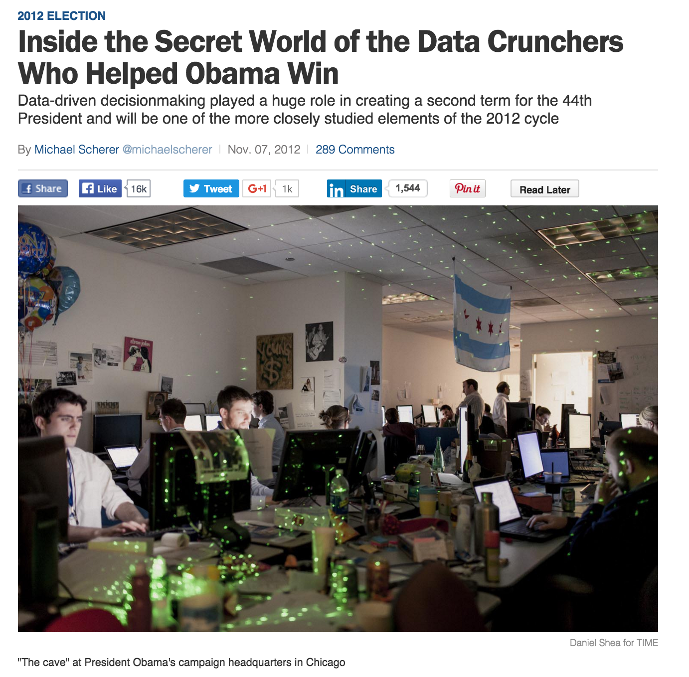
Presidential Election
Redskins Rule
If the Redskins win their final home game -> incumbent wins
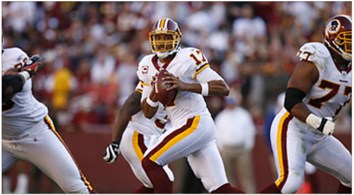
Since 1936, but not 2004 and 2012 (18-2)
LA Lakers Law
If LA reaches championship Republican wins
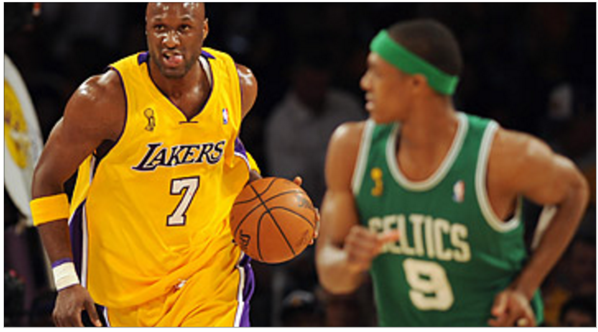
Since move to LA in 1960, but not 2008 and 2012 (12-2)
Tide vs Tigers
Alabama (D) vs LSU (R)
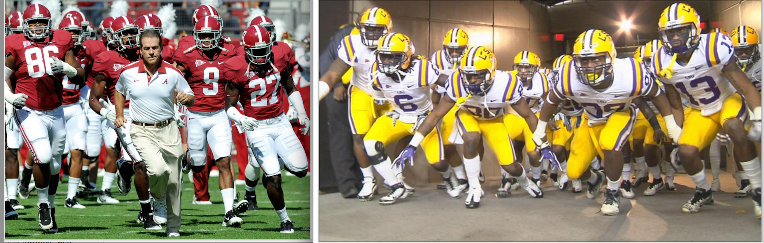
Worked since 1984 (8-0)
Family Circle First Lady Cookie Contest
Winning cookie recipe wins election
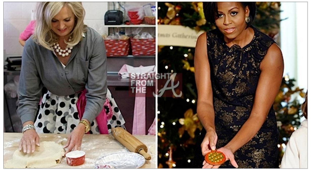
Worked since 1992, except 2008 (5-1)
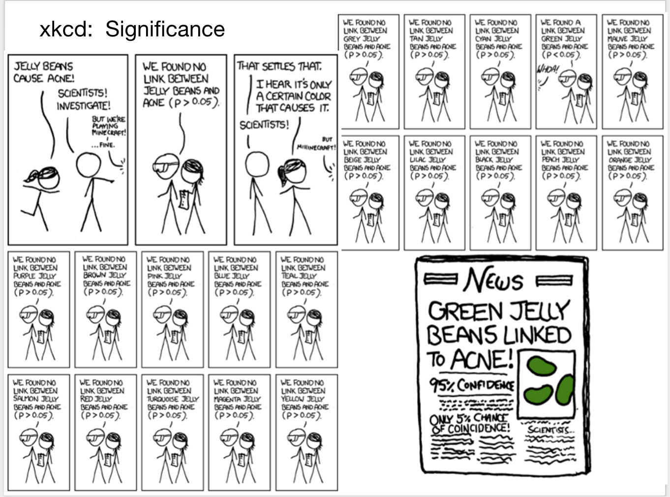
Is this a joke?
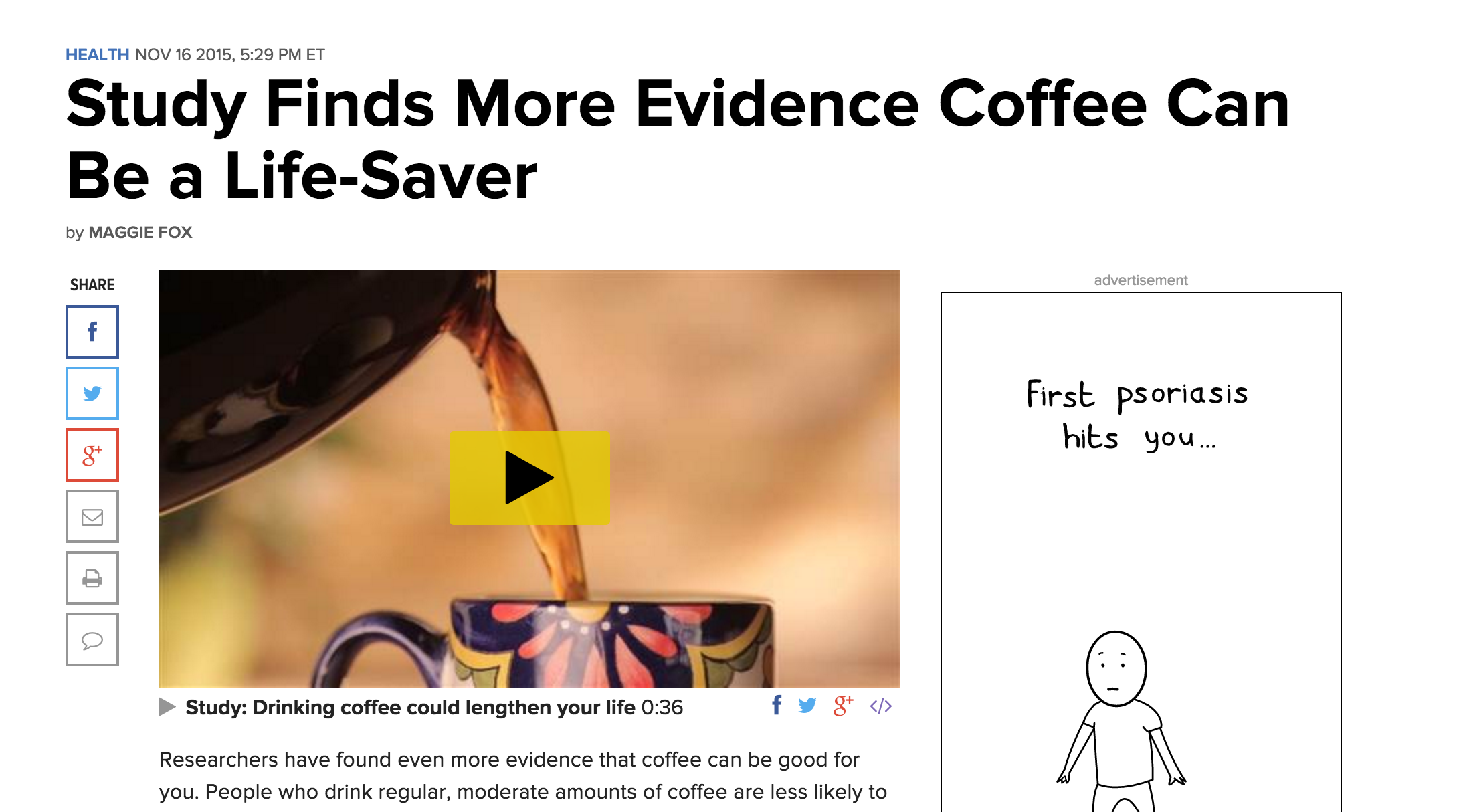
Or this?
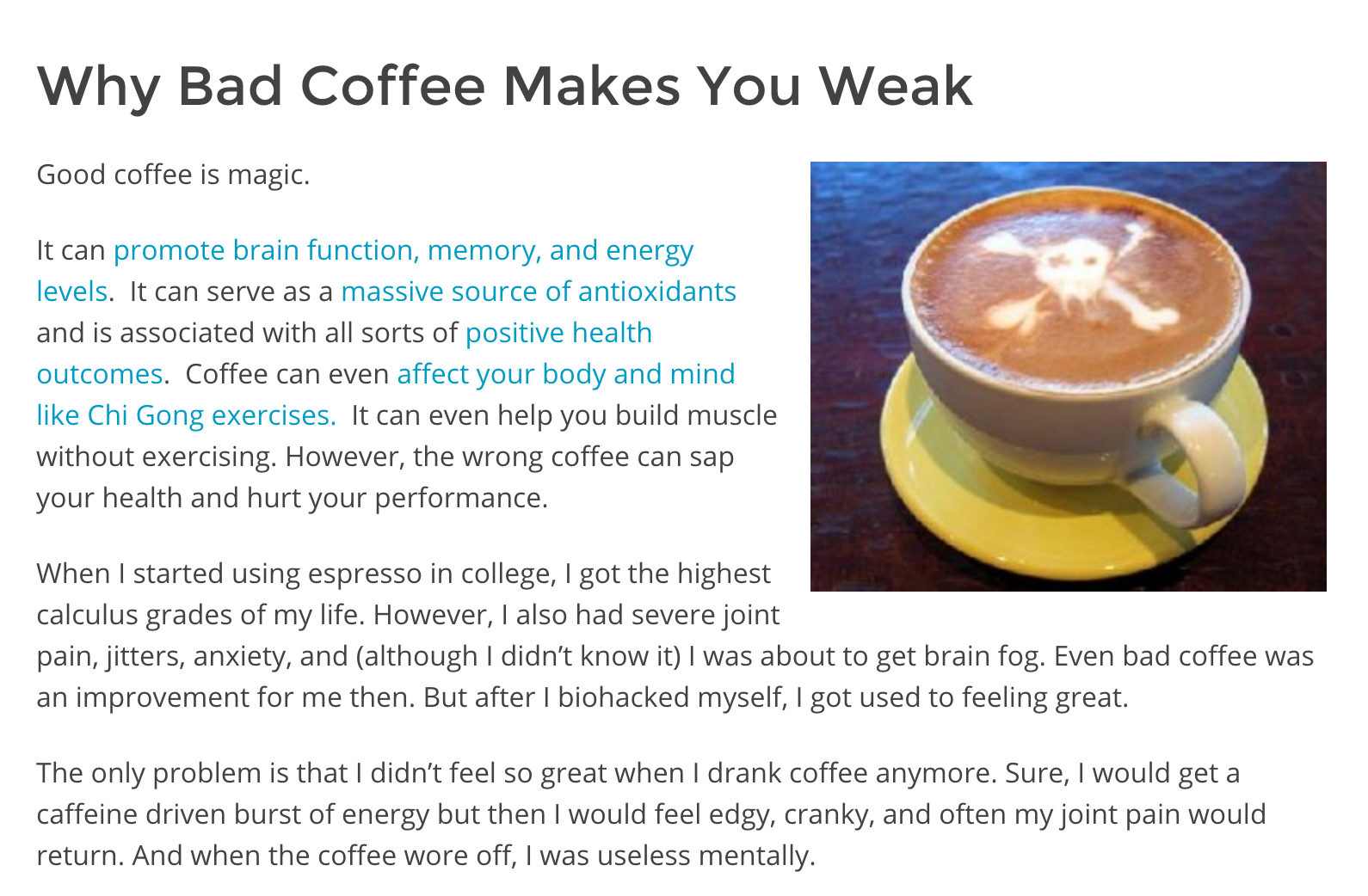
Or this?
These were not jokes
Say we are given some data
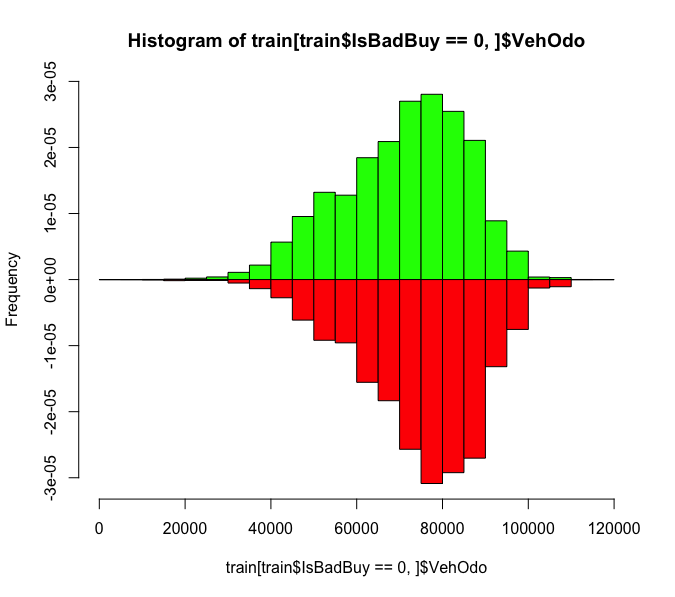
First we need to get a feel for the data
Perhaps the odometer
I don't see a huge difference
What about color?
More interesting!
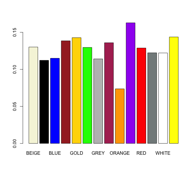
Is it statistically significant?
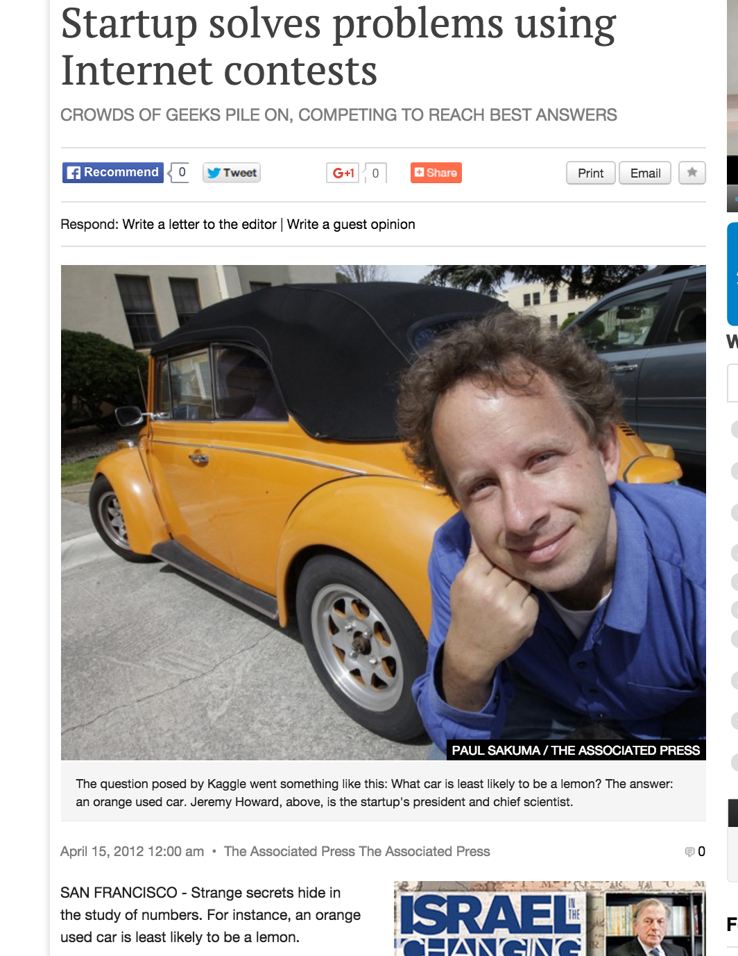
Orange Cars
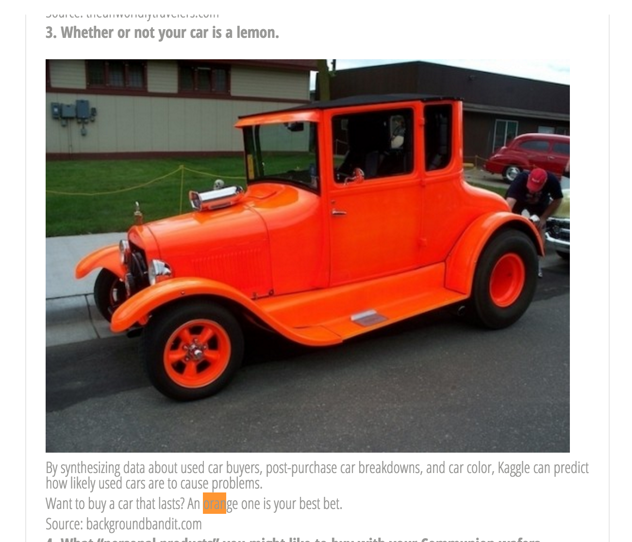
Orange Cars
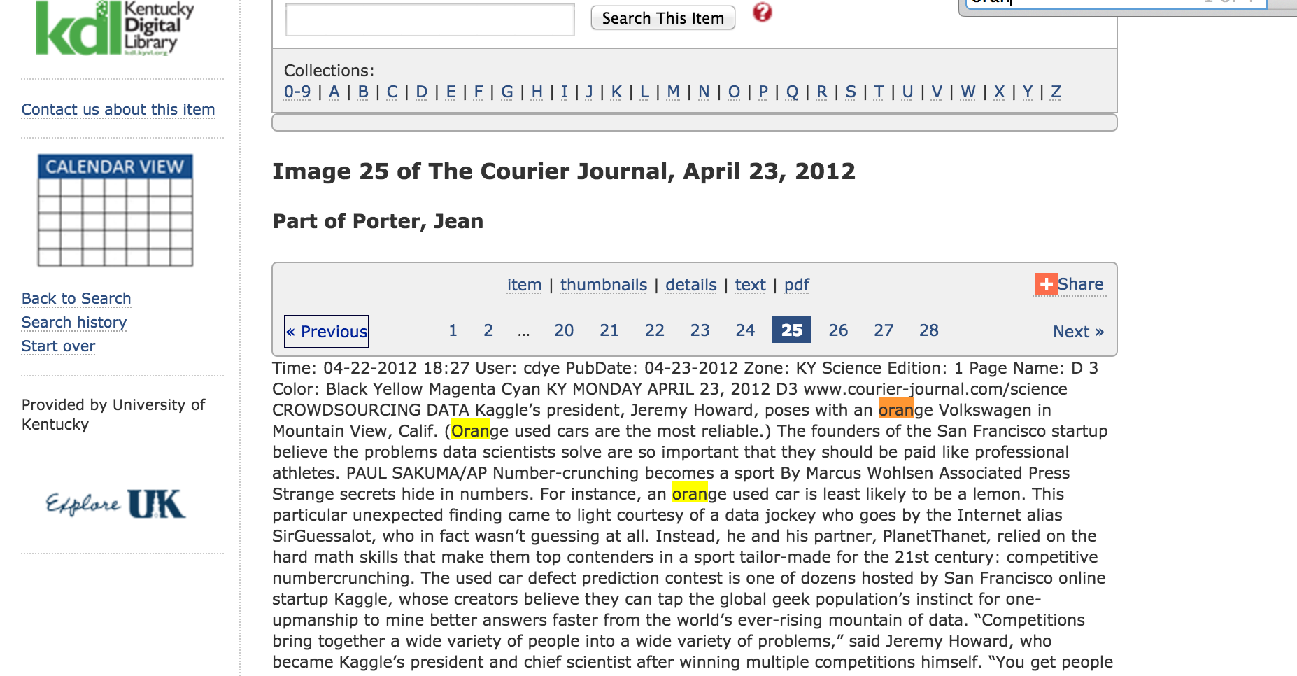
Orange Cars
To use it we would build a model
Except it was very close to random!
Target Shuffling
Not as significant as our initial result
So ...
Lets rewind a bit
Model with confidence!
I probably won't guess that good!
Lesson Learned
Crisis of False Research Findings