Bayesian Pokemon
Something very interesting occured to me recently. In most places you look there is some system that exists outside of what we can fully know. We use statistics to help explain these systems, and how much we can say about them. In some systems like video games this is a little different. In reality we collect data and it has some error in the collection process but in video games the randomness is just programmed to be draws from a random number generator. A recent game that is pretty interesting in its use of AR called Pokemon GO, has many such examples. There are lots places where the rules are truely random numbers because they were programmed that way. It is similar to the System ID work I used to do as an engineer, trying to determine the rules of a system by collecting data about it under different circumstances.
In Pokemon GO all Pokemon have a stat called CP which stands for combat points, roughly how strong they are in an attack. The case that I want to look into here is when you evolve a pokemon, the Pokemon you are going to evolve has an initial CP and the evolved Pokemon will have a CP that is potentially much higher. Can you determine what the CP will be before you evolve it? If so you have basically determined how the game draws its random numbers.
I collected a couple of cases of the evolution process for a Pidgey, a Pokemon that will evolve into a Pidgeotto. This is a convience sample though, as it was the easist Pokemon to catch a lot of.


data <- data.frame(cp = c(237, 241, 254, 305, 254, 212, 207, 175, 10, 10),
                   cp2 = c(452, 457, 483, 577, 482, 401, 391, 333, 15, 15))
We can do this from a frequentist perspective by using the lm linear model function found in R. We can look at the relationship to see if this will be a wise direction.
ggplot(data, aes(cp, cp2)) + geom_point()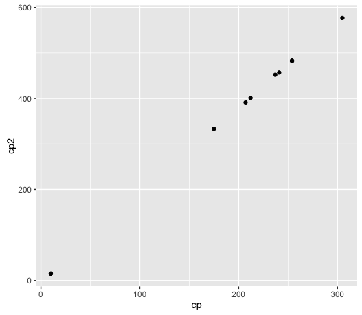
It does look like there is a linear relationship, so that is promising. We will start by doing a simple linear regression, a very common task in statistics and data science.
mod <- lm(cp2 ~ cp, data = data)
summary(mod)
##
## Call:
## lm(formula = cp2 ~ cp, data = data)
##
## Residuals:
## Min 1Q Median 3Q Max
## -2.5115 -0.6552 -0.3271 0.7449 2.4971
##
## Coefficients:
## Estimate Std. Error t value Pr(>|t|)
## (Intercept) -3.615257 1.112079 -3.251 0.0117 *
## cp 1.911891 0.005214 366.689 <2e-16 ***
## ---
## Signif. codes: 0 '***' 0.001 '**' 0.01 '*' 0.05 '.' 0.1 ' ' 1
##
## Residual standard error: 1.582 on 8 degrees of freedom
## Multiple R-squared: 0.9999, Adjusted R-squared: 0.9999
## F-statistic: 1.345e+05 on 1 and 8 DF, p-value: < 2.2e-16So it is close to double, and there is slight offset from running through the origin. It does look like a godd fit.
plot(data$cp, data$cp2)
abline(mod)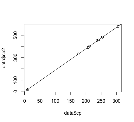
What would we predict on some new cases?
evo <- data.frame(cp = c(327, 324, 311, 184, 156, 128, 91, 77, 282, 281, 267, 218, 214, 24))

evo$f_cp2 <- predict(mod, evo)
evo
## cp f_cp2
## 1 327 621.57314
## 2 324 615.83746
## 3 311 590.98288
## 4 184 348.17271
## 5 156 294.63976
## 6 128 241.10681
## 7 91 170.36683
## 8 77 143.60036
## 9 282 535.53804
## 10 281 533.62615
## 11 267 506.85967
## 12 218 413.17701
## 13 214 405.52944
## 14 24 42.27013We can’t say much just by having these values. We can either evolve them and check or try another method to see how it contrasts to these results. What if we wanted to use a Bayesian appraoch? We could use something like Stan.
X <- model.matrix(~cp ,data)

new_X <- model.matrix(~cp, evo)
Once we have the inputs in the correct matrix form we need to construct the model. To do this using Stan we have a seperate text file that has its own syntax. It is very similar to optimzation toolkits like AMPL where you code your model in a DSL. Here we are using R as the interface to run call the stan compiler and run the model.
data {
  int N;
  int N2;
  real y[N];
  matrix[N, 2] X;
  matrix[N2, 2] new_X;
}
parameters {
  vector[2] beta;
  real sigma;
}
transformed parameters {
  vector[N] linpred;
  linpred <- X * beta;
}
model {
  beta[1] ~ uniform(-10, 10);
  beta[2] ~ uniform(0, 10);

  y ~ normal(linpred, sigma);
}
generated quantities {
  vector[N2] y_pred;
  y_pred <- new_X*beta;
}
The way we call this is by giving the stan function the text file as an arguemt and then each of the input we declared need values.
b_pok <- stan(file = "poke.stan",
               data = list(N = nrow(data), N2 = nrow(new_X),
                           K = 2, y = data$cp2, X = X,
                           new_X = new_X),
               pars = c("beta","sigma","y_pred"))
We can create and check the trace plots, which is a common practice in any Bayesian approach.
post_beta <- As.mcmc.list(b_pok, pars = "beta")
plot(post_beta)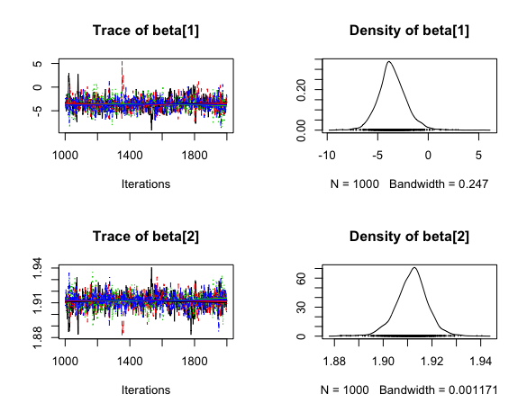
They seem pretty similar to the other appraoch.
summary(b_pok)$summary[1:2, 1]## beta[1] beta[2]
## -3.565664 1.911700mod$coefficients## (Intercept) cp
## -3.615257 1.911891What about the predictions?
evo$b_cp2 <- summary(b_pok)$summary[4:(3 + nrow(evo)), 1]Now for the real values!
evo$cp2 <- c(625, 612, 576, 344, 299, 242, 174, 145, 538, 528, 500, 408, 402, 46)evo## cp f_cp2 b_cp2 cp2
## 1 327 621.57314 621.56028 625
## 2 324 615.83746 615.82518 612
## 3 311 590.98288 590.97308 576
## 4 184 348.17271 348.18716 344
## 5 156 294.63976 294.65956 299
## 6 128 241.10681 241.13195 242
## 7 91 170.36683 170.39905 174
## 8 77 143.60036 143.63525 145
## 9 282 535.53804 535.53378 538
## 10 281 533.62615 533.62208 528
## 11 267 506.85967 506.85827 500
## 12 218 413.17701 413.18497 408
## 13 214 405.52944 405.53817 402
## 14 24 42.27013 42.31514 46These look pretty good, they are close. But looking at the standard deviation of each prediction is somewhat interesting!
summary(b_pok)$summary[4:(3 + nrow(evo)), 3, drop = F]## sd
## y_pred[1] 1.1060263
## y_pred[2] 1.0898468
## y_pred[3] 1.0211542
## y_pred[4] 0.6250458
## y_pred[5] 0.6584406
## y_pred[6] 0.7374497
## y_pred[7] 0.8904989
## y_pred[8] 0.9581057
## y_pred[9] 0.8784345
## y_pred[10] 0.8738356
## y_pred[11] 0.8122804
## y_pred[12] 0.6551967
## y_pred[13] 0.6477509
## y_pred[14] 1.2424962plot(evo$cp, summary(b_pok)$summary[4:(3 + nrow(evo)), 3], ylab = 'Residual')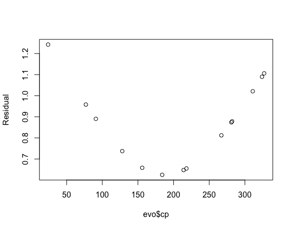
We have a huge gap in our data. It is easy to miss that when you look at the scatter plot, you are so quickly drawn to the linear relationship you glance over this issue.
plot(data$cp2, seq(data$cp2))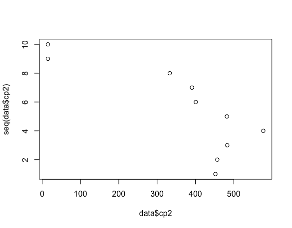
A few things come to mind here. Maybe it would help if this was done in an online manner. I don’t know if just having one value in the gap when would suffice or if I need many points. We could build a model on all of the data, since it would have fewer gaps in the input domain. Would our beta coefficiaients move any?
data2 <- rbind(data, evo[, c('cp', 'cp2')])

ggplot(data2, aes(cp, cp2)) + geom_point()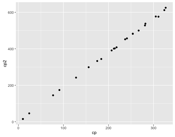
mod <- lm(cp2 ~ cp, data = data2)
summary(mod)
##
## Call:
## lm(formula = cp2 ~ cp, data = data2)
##
## Residuals:
## Min 1Q Median 3Q Max
## -11.9560 -2.9189 0.4691 2.6223 6.7430
##
## Coefficients:
## Estimate Std. Error t value Pr(>|t|)
## (Intercept) -1.019178 1.919705 -0.531 0.601
## cp 1.893811 0.008672 218.374 <2e-16 ***
## ---
## Signif. codes: 0 '***' 0.001 '**' 0.01 '*' 0.05 '.' 0.1 ' ' 1
##
## Residual standard error: 4.071 on 22 degrees of freedom
## Multiple R-squared: 0.9995, Adjusted R-squared: 0.9995
## F-statistic: 4.769e+04 on 1 and 22 DF, p-value: < 2.2e-16The y-intercept has moved closer to zero. I dont have many data points bunched up which could be an issue. I am very interested in an online or even active approach. The online appraoch would give me a new model after each evolution that took place, perhaps even indicating when you could stop with the training. An active appraoch would indicate which observation it would like to realize next, so it may converge faster.
There is also a calculator here, and it does all Pokemon. I added the ones that were predicted to our data.frame. We can use a typical evaluation strategy called root mean sqaure error (RMSE).
evo$site <- c(628, 622, 597, 353, 300, 246, 175, 148, 541, 540, 513, 419, 411, 46)

sum(sqrt((evo$b_cp2 - evo$cp2)^2))
## [1] 63.9539sum(sqrt((evo$site - evo$cp2)^2))## [1] 100It looks like both the Bayesian and Frequentist approaches do better than this site. We can do a System ID on the site as well to see how they make their predictions.
m2 <- lm(site ~ cp, data = evo)

round(predict(m2, data.frame(cp = 200)))
## 1
## 384round(predict(m2, data.frame(cp = 400)))## 1
## 768round(predict(m2, data.frame(cp = 600)))## 1
## 1152And we get the same answer they do, so this must be roughly the equation they are using to make predictions.