Markov Clustering and Voronoi

Introduction

I have used the Capital Bikeshare data to investigate a few ideas in the past and it has worked out quite well. It is a pretty useful set of data for exploring algorithms and ideas. One thing that I have been interested in lately has been how to cluster sequences. What I mean by this is how do I take something that moves from one state or place to another over some range of time and find groups of locations that entities oscillate between frequently.

I found an interesting package that does this using Markov Chains. I was already thinking that this would be an interesting approach. In the process of googling around to find some info to get started I found a package that has already done this. The package is called MCL and you an find more info about it here.

So lets dive in. Read the file, and keep relevant data. I really like how easy dplyr makes it to clean data. It is both fast, minimal and intutitive.

options(stringsAsFactors = FALSE)
library(dplyr)
library(lubridate)
library(ggplot2)
library(MCL) 
library(xml2)

'2014-Q2-Trips-History-Data.csv' %>% 
  read.csv %>%
  select(sdate = Start.date, edate = End.date, 
         sterm = Start.terminal, eterm = End.terminal, 
         bike  = Bike., type  = Subscriber.Type) %>% 
  filter(type == 'Registered') -> bike 

In order to run this algorithm we need to convert this data into a different form. We currently have it in a transactional form.

head(bike)

##             sdate         edate sterm eterm   bike       type
## 1 6/30/2014 23:59 7/1/2014 0:12 31254 31623 W21070 Registered
## 2 6/30/2014 23:56 7/1/2014 0:00 31264 31232 W20474 Registered
## 3 6/30/2014 23:56 7/1/2014 0:04 31201 31509 W20754 Registered
## 4 6/30/2014 23:55 7/1/2014 0:16 31111 31631 W21057 Registered
## 5 6/30/2014 23:55 7/1/2014 0:01 31233 31203 W21192 Registered
## 6 6/30/2014 23:54 7/1/2014 0:03 31227 31268 W20220 Registered

You can see we have when and where the trip started and ended. We also have which bike it was and the type of account the user has. The first thing we need to do is get a list of the terminals in the data set.

c(bike$sterm, bike$eterm) %>% unique %>% na.omit -> term

With this list of terminals and the trip data we need to create a transition matrix. This means we need a square matrix that has each terminal as a row and column. The simplest way to do this, not the most efficient, is to initialize a matrix of all zeros and loop through each terminal and add the the count for each destination given that starting terminal. This will take a minute.

# This initializes the transition matrix
t_mat <- matrix(0, ncol = length(term), nrow = length(term))

# Loop to get count of all station to station trips.
for (i in 1:length(term)) {
  # Subset local dataset for speed.
  tmp <- bike[bike$sterm == term[i], ]
  t_mat[i, ] <- sapply(term, function(x) sum(tmp$eterm == x, na.rm = T))
}

Now we are ready to use the MCL package.

clus <- mcl(t_mat, F)

We get three things from this function. We get the number of clusters it creates, which makes it much more useful than something like k-means clustering where we need to have some idea before hand as to how many clusters there should be in the data. We also get the number of iterations it took to to converge and the actual cluster which a terminal belongs.

clus

## $K
## [1] 17
## 
## $n.iterations
## [1] 23
## 
## $Cluster
##   [1]  4  1  4  4  4  4  4  1  1  4  4  4  4  1  1  1  0  4  1  1  4  4  3
##  [24]  1  4  4  7  4  4  4  4  4  4  1  4  4  9  7  7  4  1  4  1  1  1  4
##  [47]  4  4  4  4  1  7  4  4  4  3  4  4  1  4  6  4  4  4  4  4  4  1  1
##  [70]  5  7  1  1  1  1  1  6  1  7  4  1  7  4  4  9  4  4  4  1  4  4  4
##  [93]  9  4  1  9  1 12  1  4  3  3  1  1  7  4 12  4  1  1  3  4  1  4  1
## [116]  4  1  1  1  4  1  9  4 11  1 12  1  1  4  1  1  1  1  9  4  8  3 11
## [139]  1  7  1  1  4  9  4  8  3  4  9  1  1  3  1  1 10  4  4  7  4  1  9
## [162]  1  1  1 10  4  1 10  6  1  1  7  9 12  9  4  7  6  4  4  7  4  4  1
## [185]  4 10  9  1  3  1 11 10  3  9  4  5  4  9  9  3  1 10  1  5  4  7  5
## [208]  3  1  3  4 11  6 11  1  1  7  3  6  5  9  7 10 10  9  3 10  3 15  1
## [231]  6  1  4 13 14  5  4 10  7  5 12  3  6 14  3 14  7 11 14  7  7 12 11
## [254]  5  3  6  8 12  8  3  6  5  7  1 13  7 12  6  1  1  3 14  6  7 14 12
## [277] 14  1  5  7  7  5  3 12  1  3 12 11 17 14 10  6  6  6  5 15 16 13  1
## [300]  3  7  6  5  7 16 12 14  7  6 14 17 14  1 17 15 17 14 14 14 14  0

Lets add this new piece of information to the terminals.

station <- data.frame(terminalName = as.character(term), 
                      clus_id = clus$Cluster)

We are also quite lucky here for a few reasons. Many things that have this type of sequence where they bounce around in a manner akin to a Markov Chain are hard to plot. There are a few ways but mostly I have seen it done by actually coloring the Markov Chain nodes. Since these are locations we could plot them on a map. We are also lucky that there is a source provided that will give us the coordinates to plot each terminal on a map. Here is a function that will get the live data from each of the terminals, how many bikes are at each among other useful info, but for now we just need the latitude and longitude of each terminal.

get_locs <- function() {
  # Get data from web with locations
  'http://www.capitalbikeshare.com/data/stations/bikeStations.xml' %>%
    read_xml %>%
    xml_find_all('.//station') -> stations
  
  . %>% paste0('.//', .) %>% xml_find_all(stations, .) %>% xml_text -> get_vals
  
  c('terminalName', 'lat', 'long', 'nbBikes', 
    'nbEmptyDocks', 'lastCommWithServer') %>%
    sapply(get_vals) %>% 
    data.frame %>% 
    filter(terminalName != "8D OPS test") %>%
    mutate(lat = as.numeric(lat), long = as.numeric(long))
}

We can join this data with our above cluster data in order to plot it.

get_locs() %>% 
  select(terminalName, lat, long) %>%
  inner_join(station, by = 'terminalName') %>%
  na.omit() -> stations 

This stations data set is in a pretty tidy format now and is ready to be visualized.

head(stations)

##   terminalName      lat      long clus_id
## 1        31000 38.85610 -77.05120       7
## 2        31001 38.85725 -77.05332       7
## 3        31002 38.85640 -77.04920       7
## 4        31003 38.86017 -77.04959       7
## 5        31004 38.85787 -77.05949       7
## 6        31005 38.86230 -77.05994       7

We can use the the geom_point function and color by cluster.

ggplot(stations, aes(long, lat)) + geom_point(aes(colour = factor(clus_id)))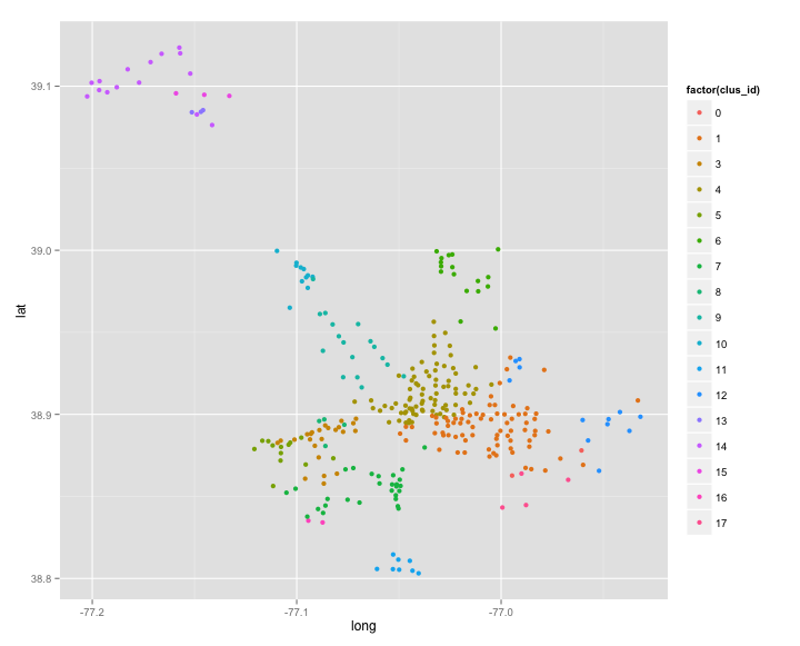

From a qualitative perspective this looks pretty good. Regions that are further away from each other tend to create there own clusters. You can also see of the roads that people travel on. I think a cool source of data to add to this would be metro loactions. Are clusters centered around these. Peole get off the metro and bike to there job?

This data has another interesting feature that I thought would be interesting to exploit. The main data file was constructed from a time period of three months in 2014. The location data comes from a live source that has terminals that did not exist then. We thus have new stations.

# Which ones have been added over the last year.
geo <- get_locs()[, 1:5]
geo[!geo$terminalName %in% stations$terminalName, ]

##     terminalName      lat      long nbBikes nbEmptyDocks
## 321        31314 38.90358 -77.06779       8            9
## 322        31081 38.80438 -77.06087       8            7
## 323        31079 38.89494 -77.09169       6            9
## 324        31078 38.86944 -77.10450       5            5
## 325        31274 38.89840 -77.02428      14            8
## 326        31080 38.89761 -77.08085       6            8
## 327        31275 38.90176 -77.05108       3           16
## 328        31082 38.80111 -77.06895       9            5
## 329        31083 38.82175 -77.04749       9            2
## 330        31084 38.80268 -77.06356       5           14
## 331        31085 38.82006 -77.05762       4            7
## 332        31086 38.82595 -77.05854       9            6
## 333        31087 38.82093 -77.05310       9            5
## 334        31088 38.83308 -77.05982       5           10
## 335        31089 38.89061 -77.08480       8           13
## 336        32049 38.98674 -77.00003       8            7
## 337        31090 38.86470 -77.04867       7            7
## 338        31315 38.96497 -77.07595       9           10
## 339        31276 38.90381 -77.03493       0           22
## 340        31277 38.89841 -77.03962      11           19
## 341        32050 38.99765 -77.03450       5           10
## 342        31278 38.91265 -77.04183       6           12
## 343        31091 38.85925 -77.06328       9            5
## 344        31517 38.90801 -76.99698       9           14
## 345        31092 38.89593 -77.10525       5           10
## 346        31093 38.89898 -77.07832       5           10
## 347        31094 38.89538 -77.09713      10            5
## 348        31279 38.89841 -77.04318      10           13
## 349        31095 38.86247 -77.06824      10            5
## 350        31280 38.91376 -77.02702       7           16

new <- merge(geo, station, all = T)
new$new <- ifelse(is.na(new$clus_id), 1, 0)

Here we can gt a look at where the new stations were added.

ggplot(new, aes(long, lat)) + geom_point(aes(colour = factor(new)))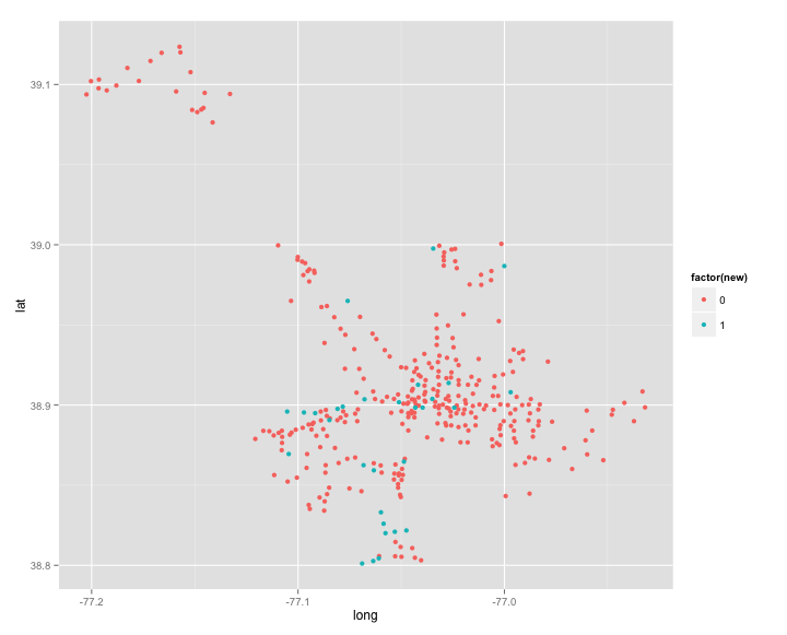

Mike Bostock wrote a great post that gave me plenty of inspiration for this. Could we see how effectively the new stations are placed. We can create a Voronoi Diagram from this and see if the distributions of areas decreases with the new stations. I found two different packages that do this in R, so i figured I would try both of them out.

library(deldir)
library(tripack)

par(mfrow = c(1, 2))

stations %>% select(x = long, y = lat) -> before
get_locs() %>% select(x = long, y = lat) -> after

plot(tile.list(deldir(before$x, before$y)), close = TRUE)
plot(tile.list(deldir(after$x, after$y)), close = TRUE)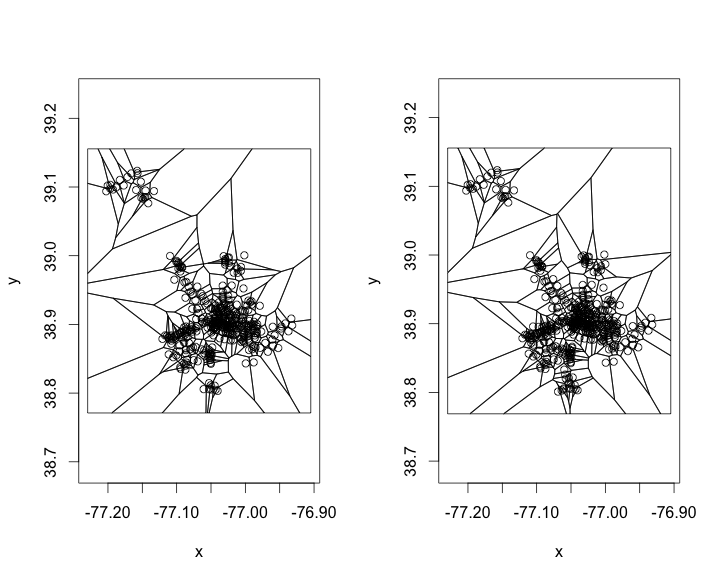

plot(voronoi.mosaic(before$x, before$y, duplicate = "error"))
plot(voronoi.mosaic(after$x, after$y, duplicate = "error"))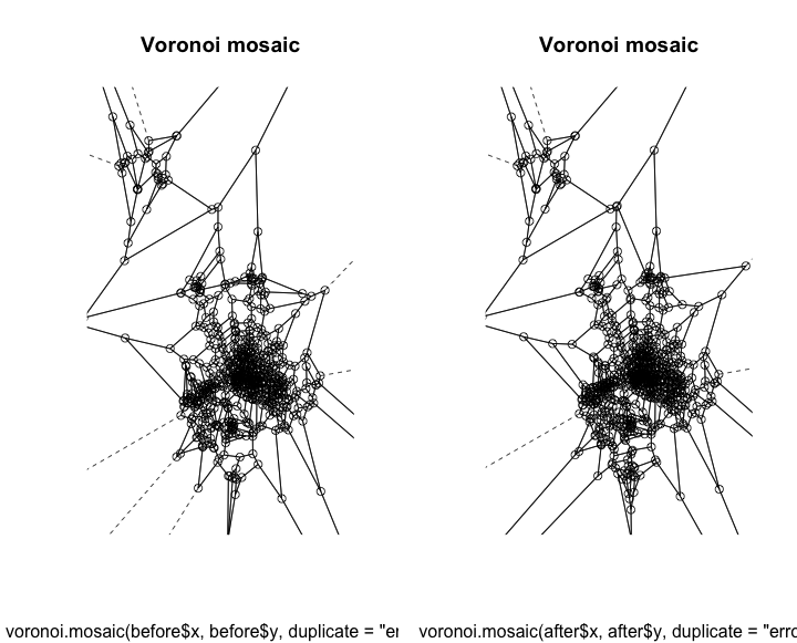

We can only see slight differences in both of them. After seeing these I have two different thoughts

This approach is not valid because they really should not be uniformly distributed. There are places where there is a greater need, even though they already have a station fairly close. The second thought is that these both look pretty rough. Even though this is not needed this is a plot that I think would work much better in d3.

To do this I need to write the data out to a csv file.

norm <- function(v) (v - min(v)) / (max(v) - min(v))

tile.list(deldir(before$x, before$y)) %>%
  lapply(function(x) data.frame(x = x$x, y = x$y)) %>%
  bind_rows %>%
  unique %>%
  mutate(x = norm(x), y = norm(y)) %>%
  write.csv(file = 'before.csv', row.names = F)