A few months back I attended the DC Open Data Day. It was a pretty interesting event and hackathon. There were a lot of interesting problems. You can get an overview of some of the stuff we worked on here.
I want to walk through some of this to address a common problem in data science. Here are some of the initializations you will need to follow along.
library(rvest)
library(dplyr)
library(leaflet)
library(igraph)
library(VennDiagram)

# This makes reading data in from text files much more logical.
options(stringsAsFactors = FALSE)
To get the data you can go to the GTFS website. There are many locations where this data is collected from. I have created a pretty simple way to get some of it.
To do this we first create functions to crawl the site and find the locations of all of the sources zip files.
# This function gets all of the URLs on the main page.
# The link to each location where data is contained.
get_all_urls <- function() {
  'http://www.gtfs-data-exchange.com/agencies' %>%
    html() %>% html_nodes('a') %>%
    html_attr('href') %>%
    grep('agency', ., value = T) %>%
    paste0('http://www.gtfs-data-exchange.com', .) -> locations

  # Last one is check
  locations[-length(locations)]
}

# This function will get the url for the zip file.
. %>% html() %>%
  html_nodes('a') %>%
  html_attr('href') %>%
  grep('.zip', ., value = T) %>%
  grep('agency', ., value = T) %>%
  paste0('http://www.gtfs-data-exchange.com', .) -> get_zip_url
Now we can get a list of all of the cities. This will take a minute so we can just get a few of them. We also need a function to go to each site to download the the actual zip file.
all_zips <- lapply(get_all_urls()[1:3], get_zip_url)

# Function to download a zip file, unzip it and move text files around.
download_gtfs <- function(url, loc) {
  download.file(url = url, destfile = paste(loc, basename(url), sep = '/'))

  name <- gsub('http://www.gtfs-data-exchange.com/agency', loc, url)
  name <- gsub('/latest.zip', '', name)
  # Unzip downloaded file
  url %>% basename %>% paste(loc, ., sep = '/') %>% unzip(., exdir = name)
  unlink(paste(loc, basename(url), sep = '/'))
}
To use this we need to create a folder to store the data. For speed and space reasons lets just grab one of the locations data.
dir.create('gtfs_data')
download_gtfs(all_zips[[1]], 'gtfs_data/')
Once we have a folder of data from one location what do we do. This is often a problem whether you get access to a database, and excel file with many worksheets or as we have here a folder with a collection of flat files. How do we figure out the structure of this data. This took some time each of us to understand how these tables were put together and how they were related. The issue I want to tackle here is the relations.
We can run this code to help with this.
The first thing we do is use the Get.Files function pointed at the folder with text files. This actually reads the data into a list of data.frames. Then we can run the Learn.Schema function on the list of data.
gtfs_data <- Get.Files('gtfs_data/a-reich-gmbh-busbetrieb/', delim = ',')

schema <- Learn.Schema(gtfs_data)

plot(schema[[2]])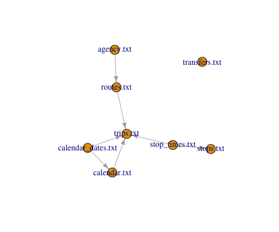
We have one file that is really not related to the rest. We can confirm what we have seen and drop it using Not.Connected and Drop.Extremes.
Not.Connected(schema[[2]])## [[1]]
## IGRAPH DN-- 7 7 --
## + attr: name (v/c), col (e/c)
## + edges (vertex names):
## [1] agency.txt ->routes.txt calendar_dates.txt->calendar.txt
## [3] calendar_dates.txt->trips.txt calendar.txt ->trips.txt
## [5] routes.txt ->trips.txt stop_times.txt ->stops.txt
## [7] stop_times.txt ->trips.txt
##
## [[2]]
## [1] "transfers.txt"schema[[2]] <- Drop.Extremes(schema[[2]])
plot(schema[[2]])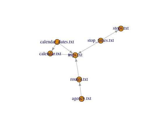
This is now pretty useful, we can see the larger organization of this data, mainly how we could join one table onto another. We can see what fields we would join on by what they have in common.
d <- schema[[1]]
d
## x y z
## 1 agency.txt routes.txt agency_id
## 2 calendar_dates.txt calendar.txt service_id
## 3 calendar_dates.txt trips.txt service_id
## 4 calendar.txt trips.txt service_id
## 5 routes.txt trips.txt route_id
## 6 stop_times.txt stops.txt stop_id
## 7 stop_times.txt trips.txt trip_idThe next thing to check for is the actual overlap of these fields. Does one table contain everything and the other a subset or does neither contian every unique observation from a certain field.
d$a <- NA
d$b <- NA
d$c <- NA


for (i in 1:nrow(d)) {
  a <- gtfs_data[[d[i, 1]]][, d[i, 3]]
  b <- gtfs_data[[d[i, 2]]][, d[i, 3]]

  d$a[i] <- length(unique(a))
  d$b[i] <- length(unique(b))
  d$c[i] <- length(intersect(a, b))
}

d
## x y z a b c
## 1 agency.txt routes.txt agency_id 142 54 54
## 2 calendar_dates.txt calendar.txt service_id 1779 1778 1778
## 3 calendar_dates.txt trips.txt service_id 1779 1126 1126
## 4 calendar.txt trips.txt service_id 1778 1126 1126
## 5 routes.txt trips.txt route_id 1336 1336 1336
## 6 stop_times.txt stops.txt stop_id 12812 12812 12812
## 7 stop_times.txt trips.txt trip_id 282754 282754 282754field <- 'agency_id'
x <- d[d[, 'z'] == field, ]
x <- unique(c(x$x, x$y))
a <- unique(gtfs_data[[x[1]]][, field])
b <- unique(gtfs_data[[x[2]]][, field])
ab <- length(intersect(a, b))This looks good as everything is a subset of some other full set.
draw.pairwise.venn(length(a), length(b), length(intersect(a, b)),
                   category = c(x[1], x[2]),
                   fill = c("goldenrod1", "darkorange1"),
                   cat.col = c("goldenrod1", "darkorange1"), cat.cex = 2)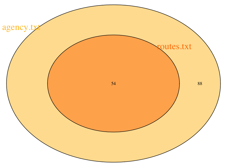
Here we can see how one is completely contained inside the other. We can also use this info to figure out how to merge these sources together to get some set of data that is more insteresting.
# Read the files into R.
routes     <- read.csv("gtfs_data/a-reich-gmbh-busbetrieb/routes.txt")
stop_times <- read.csv("gtfs_data/a-reich-gmbh-busbetrieb/stop_times.txt")
stops      <- read.csv("gtfs_data/a-reich-gmbh-busbetrieb/stops.txt")
trips      <- read.csv("gtfs_data/a-reich-gmbh-busbetrieb/trips.txt")


# Join the data together.
stops %>%
  inner_join(stop_times, by = "stop_id") %>%
  inner_join(trips, by = "trip_id") %>%
  inner_join(routes, by = "route_id") %>%
  select(stop_id, trip_id, route_id, stop_lon, stop_lat) -> data


data[data$trip_id == data$trip_id[1], ] %>% arrange(route_id) -> ro1


(leaflet() %>% addTiles() %>%
   setView(lng = ro1$stop_lon[1], lat = ro1$stop_lat[1], zoom = 10) %>%
   addCircles(color = 'black', lat = ro1$stop_lat, lng = ro1$stop_lon))