MMA Predictions Using SNA
Kenny Darrell
November 18, 2014
History
Mixed Martial Arts (MMA) is a newer sport, but it has grown pretty fast. I remember being young and seeing advertisements for the first UFC event. Being a kid from the eighties who enjoyed professional wrestling I was pretty fascinated. It was a different beast back then in the early nineties though. It has evolved into a very large and organized sport. There are also different organizations in this realm, Bellator, PRIDE and UFC.
For many reasons this interests me. If you have read any of my past blogs you can see lots of topics related to sports. My other interests of temporal data and network data are both very relevant here. It is also an area that allows for a model to be built in order to predict outcomes, and unlike many other sports the clock does not reset after every season, they can exist outside of that notion. They also allow for some great visualizations as well as just an interesting problem to work on.
Collecting Data
There are quite a few sources for information in this area. Some are pretty explicit about not scraping data and others seem to be more open. There is a lot of data on ESPN. To pull this data I used the new rvest package which made things very easy compared to other methods I have used in the past. I tried to use some of the newer web-scraping tools but ran into some issues. I hope that these tools continue to evolve, and perhaps I should retry or try others to see which ones are more capable, perhaps a blog for another day.
Using rvest and dplyr together makes the code look like a pipeline, very clean and readable. Here you can see how you would go about getting which fighters exist, who they have fought and some of there metadata.
'http://espn.go.com/mma/fighters' %>%
  html() %>%
  html_nodes('.evenrow, a') %>%
  html_attrs() %>%
  grep('/fighter/', ., value = T) %>%
  sapply(function(x) x[[1]]) %>%
  as.character() %>%
  head()
## [1] "/mma/fighter/_/id/3043549/niina-aaltonen"
## [2] "/mma/fighter/_/id/2504991/tom-aaron"
## [3] "/mma/fighter/_/id/3088828/joshua-aarons"
## [4] "/mma/fighter/_/id/3089919/mike-aarts"
## [5] "/mma/fighter/_/id/2511451/zyad-abada"
## [6] "/mma/fighter/_/id/2966179/kadzhik-abadzhyan"'http://espn.go.com/mma/fighter/history/_/id/3031574/matthew-lozano' %>%
html() %>%
html_nodes('div div div .evenrow td') %>%
html_text() %>%
matrix(ncol = 7, byrow = T) %>%
data.frame() %>%
select(date = X1, opponent = X3, result = X4, method = X5, time = X7)## date opponent result method time
## 1 Oct 11, 2013 Klayton Mai Win Submission (Triangle Choke) 1:14
## 2 Oct 19, 2012 Dave Morgan Win Submission (Triangle Choke) 2:28
## 3 Jun 29, 2012 Joshua Aarons Win Submission (Triangle Choke) 4:23'http://espn.go.com/mma/fighter/stats/_/id/3031574/matthew-lozano' %>%
html() %>%
html_nodes('.general-info li') %>%
html_text()## [1] "Bantamweight" "5'7\", 135 lbs."You can set up a process to pull the data in its entirety by putting a few loops or lapply functions around the above code. You then need to clean it up a bit and get it into a tidy data format.
head(fights)## id date opp result round time
## 1 3032062 2011-09-03 eduard folayang Loss 3 5:00
## 2 3032062 2010-09-24 guangyou ning Win 3 5:00
## 3 3050604 2010-02-21 john robles Loss 1 0:48
## 4 2557041 2009-08-15 francisco rivera Loss 3 5:00
## 5 2499256 2004-12-18 dan hardy Loss 1 0:13
## 6 2504979 2010-05-07 keto allen Loss 1 2:58The first thing that I thought would be useful is to build a model that can predict the outcome of a given fight. There are a few reasons why this problem is different than building a typical model. The most important reason is that each observation is not independent. This lack of independence happens on many levels. First if I have a fight to predict I actually have it setup as two fights now, one for each fighter. I cannot predict the outcome of the fight like this, What if I have a model that says both fighters win. There is also a larger network effect, any given fight could have fighters that have fought in many other fights, maybe even a clone of the fight under consideration. It also leaves us with no data about the opponent which is a real challenge.
Restructure
The first step is to resolve the issue of each fight really having two different observations, one from each side. I started writing code to this and it turned out to be very, very gross. It was hard to grapple in my head. Weird things had to happen, I had to join the data on itself but change the names of fields to get over the collision of the fighter attributes. One thing I want to address here, which I have spoke about some in the past is using the right tool for the job. After I started down the path of trying this I realized this approach was all wrong. Here is a glimpse of what that code looked like, pretty ugly.
# Make names with winner and loser
fights$winner <- ifelse(fights$result == 'Win', fights$name, fights$opp)
fights$loser <- ifelse(fights$result == 'Loss', fights$name, fights$opp)

# Now remove opponent field
fights$opp <- NULL

# need to create two tables, one will have the data for winner and one the loser
left <- fights[fights$result == 'Win', c(1, 3:7, 2, 8:9)]
right <- fights[fights$result == 'Loss', c(1, 3:7, 2, 8:9)]

# Change the names of each to denote fields realtion.
names(left)[1:6] <- paste('wn_', names(left)[1:6], sep = '')
names(right)[1:6] <- paste('ls_', names(right)[1:6], sep = '')

left <- left[order(left$date), ]
right <- right[order(right$date), ]

# Create a table of atomic fight data.
key <- fights[, c('date', 'winner', 'loser')]
key <- unique(key)

# This joins the left and right side (winner/loser) data on
join <- merge(key, left, by = c('date', 'winner', 'loser'))
join <- merge(join, right, by = c('date', 'winner', 'loser'))

# We should have two rows for each
join <- unique(join)

# No longer have becuase we have winner and loser fields.
join$wn_name <- NULL
join$ls_name <- NULL
join$wn_result <- NULL
join$ls_result <- NULL

# Create an id for each fight
join$matchid <- as.character(1:nrow(join) + 100000)

# Cleanup tables.
rm(key, left, right)

# Now we have to merge the bio data on for both the winner and loser.
pl_lk <- data
pl_lk$name <- NULL

# Need to rename everything
names(pl_lk) <- paste('wn_', names(pl_lk), sep = '')
join2 <- merge(join, pl_lk, by = 'wn_id')

# Redo for loser and switch names
names(pl_lk) <- gsub('wn_', 'ls_', names(pl_lk))
join3 <- merge(join2, pl_lk, by = 'ls_id')

# Finally have the right structure
fight <- join3
This seems like a perfect place to use Neo4j. I can give it each fighters data and then create a relation for each fight. Then I can just query for the data I want and have it return it in the right format. Shove all of my data into Neo4j and have cypher do all of the messy parts behind the scenes, perfect.
I created some code that sits on top of the RNeo4j package so that you can add whole tables with given relationships, which there may now be some new commits that allow you to do this. I just loop through the fighter attribute data and the fight data adding everything.
graph = startGraph("http://localhost:7474/db/data/")

person <- add_nodes(data, c('fighter', 'espn'), 'id', props = names(data))

add_rels(fights, from = person, f_name = 'id', to = person, t_name = 'oppid',
         how = 'fought', props = c('date', 'result', 'dec', 'time'))
I can get the data I want by using a query like this.
MATCH (a)-[r:fought]->(b)
  WHERE r.result = "Win"
  RETURN a.name as wname, a.weight as ww, r.dec as dec, r.date as date,
         b.name as lname, b.weight as lw
UNION ALL MATCH (a)-[r:fought]->(b)
  WHERE r.result = "Loss"
  RETURN b.name as wname, b.weight as ww, r.dec as dec, r.date as date,
         a.name as lname, a.weight as lw;
I now just use the cypher function with this query passed in as a string and the data I want is returned.
fight <- unique(cypher(graph, query))Data Exploration
We now need to get some understanding of how this data looks. What about it may be useful knowledge before we try to build a model. For instance how many fights are there in a year.
fight %>% mutate(date = ymd(date), year = year(date)) -> fight

plot(table(fight$year), xlab = 'Year', ylab = '# of Fights',
     main = 'Number of Fights a Year')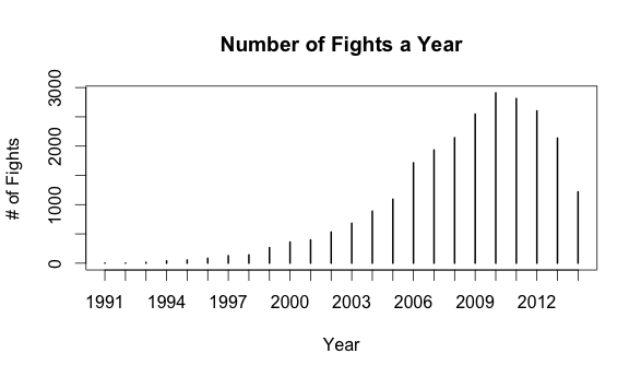
It is interesting that the number of fights has been dropping off over the past few years. From my limited exposure I have not noticed this. Maybe it is only the other leagues are starting to diminish. How would this same plot look from only the perspective of the UFC?
ufc <- fight[grep('UFC', fight$event), ]
plot(table(ufc$year), xlab = 'Year', ylab = '# of UFC Fights',
     main = 'Number of UFC Fights a Year')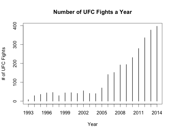
Very interesting. They seem to still be growing. Even more so considering that this plot does not have the last two months of 2014 included in the data.
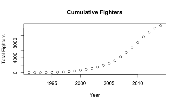
What about from the perspective of the fighters. How many MMA fighters are there?
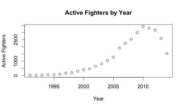
How many of these fighters are actually active in a given a year?
Missing data
Once you start digging into the data you quickly realize that there are lots of holes. Most of the predictor variables you would start with are missing. What would be the best way to resolve this? I have a few thoughts, but some require a lot more effort. Pulling data from another source that is more complete was my first thought. The problem is though that would mean starting over.
##        id           name weight height         class country birth stance
## 1 3032062     a sol kwon   <NA>   <NA>          <NA>    <NA>  <NA>   <NA>
## 2 3050604 aaron anderson   <NA>   <NA>          <NA>    <NA>  <NA>   <NA>
## 3 2557041    aaron arana    135   <NA> Featherweight    <NA>  <NA>   <NA>
## 4 2499256   aaron barrow   <NA>   <NA>  Welterweight    <NA>  <NA>   <NA>
## 5 2504979    aaron berke   <NA>   <NA>  Welterweight    <NA>  <NA>   <NA>
## 6 3010409     aaron birn   <NA>   <NA>          <NA>    <NA>  <NA>   <NA>
Two things to note. I had first hoped I could just pull data to replace everything I had done, find a source with perfect data. This did not work out. Then I thought I could pull data for another source and merge the two together. This would mean I have two partial sources, say 25% and 35% complete. Could they be resolved into one data set that is closer to 60%. The answer is no and yes. I know they will not be complete opposites, they will have some overlap, so the combination should be more than either of the parts but less than the sum. How many sources are out there? Could you merge three or more together. Would this be a diminishing returns problem? This would lead to an entity resolution problem, and a tough one at that. There are some tools to help solve this problem, but that may be a challenge for another day. It is getting close to the issue of waiting for perfect data. I think that getting more data and having a cleaner set would be valuable, but after fusing another set I may be in the same boat.
My second thought was, can I use network attributes for predictor variables. The cleanest part of the data is the collection of fights, its participants and the result. I started thinking of my posts on Social Balance. If A beats B, and B beats C should I be able to predict that A will beat C. Maybe, what if that was a long time ago. Can MMA exhibit paper rock scissors type of effects. Maybe certain styles of fighting have weaknesses to others. You could also be having an off day. This means we need to look at the network of fights. It also means that we need to look at how it evolved, not just how it exists today.
Visualizing the Network
I created a gexf file of the network that gave a temporal element to when fights occurred and when fighters were considered to be active. This network is really cool how it evolves over time. We can actually see the sport getting big. The problem is the visualization starts to fall apart. Viewing these things is a really hard problem. In this first video you can see a force directed layout algorithm moving the things around. Every few seconds another sixty days of data is pulled into the network. A fighter exists into the network from his first appearance in a fight until about 200 days after his last fight. The fight itself, depicted as the edges are only visible for a little over half a year. This way the older fights phase out. The size of the node is dependent on the pagerank of the node under consideration. There is also a thickness of the edges which denotes the value of the fight, how much it can change the nodes pagerank. This time lapse covers roughly the years of 2001 to 2007.
In this plot we have a different layout algorithm, Fruchterman-Reingold, which gives a much different feel. Everything else is the same except that the time period is around 1999 to 2003.
Here we have 2007 to 2011 with everything else being the same as above.
Create the Analytic Data Set
q <- '
MATCH (a)-[r:fought]->(b)-[s:fought]->(a)
WHERE r.result = "Win" and r.date = s.date
RETURN a.name as name, a.id as id, a.weight as weight, a.height as height,
       r.result as result, r.date as date, r.exp as exp, s.exp as oexp,
       b.id as oid, b.weight as oweight, b.height as oheight
UNION ALL
MATCH (a)-[r:fought]->(b)-[s:fought]->(a)
WHERE r.result = "Loss" and r.date = s.date
RETURN a.name as name, a.id as id, a.weight as weight, a.height as height,
       r.result as result, r.date as date, r.exp as exp, s.exp as oexp,
       b.id as oid, b.weight as oweight, b.height as oheight;'

f <- unique(cypher(graph, q))
Now we can start to create the variables we will use to build a model. My first since we will be going down the graph centric route, how do nodes fair that have zero degree. Translation, do fighters usually lose on there first fight. If so how does this change as they gain more experience.
w <- as.data.frame(table(f[f$result == 'Win', ]$exp))
l <- as.data.frame(table(f[f$result == 'Loss', ]$exp))

names(l)[2] <- 'Freq2'
winloss <- merge(w, l, all.x = T, all.y = T)
names(winloss) <- c('Experience', 'Win', 'Loss')
head(winloss, 10)
## Experience Win Loss
## 1 1 2811 9932
## 2 2 2040 3296
## 3 3 1761 1752
## 4 4 1510 1197
## 5 5 1395 893
## 6 6 1307 681
## 7 7 1218 575
## 8 8 1092 547
## 9 9 1044 486
## 10 10 945 447This seems to have some promise. Do fighters win more after they have some fights under there belt? We have not yet even considered the opponents experience. It is very interesting that only about one out of every five fighters will win there first fight. It is about two out of five will win there second and by the time you get to your third you are at about even odds. As you get further it seems to converge around two to one. There may still be more happening here though since there are many more cases in the first fight than the second. Maybe some survivor bias. If you lose your first you may not have an opportunity to have a second.
How do the other variables fare that are not network centric? We should at least evaluate them to see if it would even help to get complete data from other sources.
f$weight <- as.numeric(f$weight) - as.numeric(f$oweight)

# Weight does not seem to help much.
mean(f[f$result == 'Win', ]$weight, na.rm = T)
## [1] -1.482577sd(f[f$result == 'Win', ]$weight, na.rm = T)## [1] 17.90397f$weight <- NULL
f$oweight <- NULL
f$height <- as.numeric(f$height) - as.numeric(f$oheight)
# Height does not help either.
mean(f[f$result == 'Win', ]$height, na.rm = T)## [1] 0.1363392sd(f[f$result == 'Win', ]$height, na.rm = T)## [1] 2.749247f$height <- NULL
f$oheight <- NULL
f$birth <- NULL
f$obirth <- NULLSo it seems the variables I thought at first would be useful had very little value. I still think that there may be some value in other variables such as age and style but they are missing more often than not so. They are also other variables that I think may be useful like how you won the fight and how long it took but first I want to check out the graph measures and see how they play out. To construct the network variables we need to use some forthought.
grTab <- function(gr) {
  data.frame(        id = vertex.attributes(gr)$name,
              closeness = centralization.closeness(gr)$res,
             betweeness = betweenness(gr),
            eigenvector = centralization.evcent(gr)$vector,
                    hub = hub.score(gr)$vector,
                   auth = authority.score(gr)$vector,
                   page = page.rank(gr)$vector)
}

q2 <- 'MATCH (a)-[r:fought]->(b)
       WHERE r.result = "Win"
       RETURN a.id as id, a.name as name, r.date as date,
              b.id as oid, b.name as oname;'

q2 %>% cypher(graph, .) %>% unique() %>%
  mutate(date = ymd(date)) -> f2

time <- sort(unique(f2$date))
g <- graph.data.frame(f2[f2$date < time[10], c('oname', 'name')])

plot(g)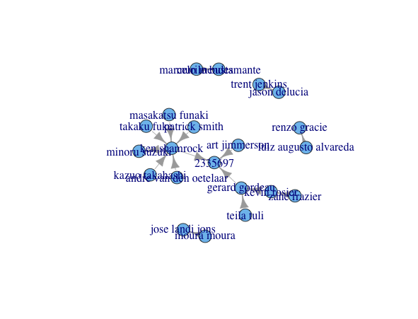
d3plot(g)We cannot just evaluate the centrality measures as they stand today. That would be a leak from the future, we would be using information to predict the outcome of a fight with information that already knows what the outcome is. Thus it is critical to step back through time, creating a new network at each point and evaluate the centraility measures. Then this data will be added back onto the correct observations.
pageRank <- list()
for (i in 2:length(time)) {

  g <- graph.data.frame(f2[f2$date < time[i], c('oid', 'id')])
  y <- x <- cbind(grTab(g), date = time[i])
  names(x) <- c("id", "cl", "bet", "eig", "hub", "auth", "page", "date")
  names(y) <- c("oid", "ocl", "obet", "oeig", "ohub", "oauth", "opage", "date")

  tmp <- f2[f2$date == time[i], ]
  tmp <- merge(tmp, x, by = c('id', 'date'), all.x = T)
  tmp <- merge(tmp, y, by = c('oid', 'date'), all.x = T)

  pageRank[[as.character(i)]] <- tmp
  print(i)
}

pageRank <- recurBind(pageRank)[[1]]

page <- pageRank[, c('page', 'opage')]
page <- page[complete.cases(page), ]
sum(page[, 1] < page[, 2])
## [1] 4052sum(page[, 1] > page[, 2])## [1] 9119I am still thinking through if this is the best way to setup this model. I am not sure what all of the implications are to make a prediction for both sides. I will move forward as is though. Now that things are ready to build a model I need to create a training and testing set. This will be done using a roughly 70/30 split. One difference is that the training data will be before a certain point in time and the testing will be after. This will enforce that both sides from a fight fall in the same split. It also enforces that there are no leaks from the future. From there we can pass the cleaned up data to the algorithm.
f3 <- f3[order(f3$date), ]

train <- f3[f3$date <= f3$date[30000], -1]
test <- f3[f3$date > f3$date[30000], -1]

mod <- randomForest(y ~ ., data = train, ntree = 100, do.trace = 1)
## | Out-of-bag |
## Tree | MSE %Var(y) |
## 1 | 0.2931 117.22 |
## 2 | 0.2806 112.25 |
## 3 | 0.265 105.99 |
## 4 | 0.2539 101.57 |
## 5 | 0.2438 97.51 |
*******************
## 96 | 0.1681 67.25 |
## 97 | 0.1681 67.24 |
## 98 | 0.168 67.20 |
## 99 | 0.168 67.20 |
## 100 | 0.168 67.19 |Now let's check how the model performs on the test data set.
eval <- as.numeric(predict(mod, newdata = test, type = 'response'))

xp <- prediction(eval, test$y)
performance(xp, 'auc')
## [1] 0.8277932plot(performance(xp, "tpr","fpr"))
points(seq(0, 1, .01), seq(0, 1, .01), type = 'l')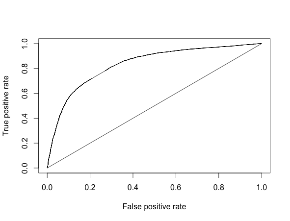
These results seem pretty good. My concern from earlier may still be valid. We can check it against data that has occurred since I collected the first sample. There has been a few events since the maximum date contained in the data set. We can check these and be completely sure that the model has some predictive ability.
max(f2$date)## [1] "2014-11-02"clean <- function(x) {
x %>% html_attrs() %>% sapply(function(x) x[[1]]) %>% as.character() %>%
gsub('http://espn.go.com/mma/fighter/_/id/', '', .) %>% strsplit('/') %>%
sapply(function(x) x[[1]][1])
}
get_event <- function(url) {
url %>% html() -> html
html %>% html_nodes('.winner') %>% html_attrs() %>%
sapply(function(x) x[[1]]) %>% strsplit(' ') %>%
sapply(function(x) x[[2]]) -> w
html %>% html_nodes('.player1 a') %>% clean() -> a
html %>% html_nodes('.player2 a') %>% clean() -> b
data.frame(winner = ifelse(w == 'fighter1', a, b),
loser = ifelse(w == 'fighter1', b, a))
}
new_pred <- function(event) {
event %>% get_event() -> ev
merge(data.frame(id = c(ev$winner, ev$loser)), f2, all.x = T) %>%
mutate(data = ymd(date)) %>%
select(id, date, exp, cl, bet, eig, hub, auth, page) %>%
group_by(id) %>%
mutate(max = max(date)) %>%
filter(max == max(date)) %>%
select(-max, -date) %>%
as.data.frame -> cc
cc[is.na(cc)] <- 0
bb <- cc
names(bb) <- paste0('o', names(bb))
rbind(select(ev, id = winner, oid = loser),
select(ev, oid = winner, id = loser)) %>%
merge(cc) %>% merge(bb) %>%
mutate(expDiff = exp - oexp, clDiff = cl - ocl, betDiff = bet - obet,
eigDiff = eig - oeig, hubDiff = hub - ohub, authDiff = auth - oauth,
pageDiff = page - opage) -> ndata
ndata$p <- predict(mod, newdata = ndata[, -c(1:2)], type = 'response')
ev %>%
merge(select(ndata, winner = id, wp = p)) %>%
merge(select(ndata, loser = id, lp = p))
}past <- c('http://espn.go.com/mma/fightcenter?eventId=400603491',
'http://espn.go.com/mma/fightcenter?eventId=400601611',
'http://espn.go.com/mma/fightcenter?eventId=400592231')
new_pred(past[1])## loser winner wp lp
## 1 2614776 3040385 0.5667222 0.4365436
## 2 2972878 2989176 0.5284568 0.5169444new_pred(past[2])## loser winner wp lp
## 1 3077213 3088238 0.6611667 0.4375436
## 2 3077809 3026147 0.5157658 0.5275556
## 3 3114205 2546733 0.5475000 0.4849880
## 4 3155286 3122040 0.7240323 0.2706634new_pred(past[3])## loser winner wp lp
## 1 3097617 3153263 0.5256547 0.4799444These look pretty good as well. It gets 6 out of 7. The only one we got wrong was very close, the model was was not really picking a side. I think I am going to let it run for a few more events before I make any real conclusions.